Mathematics – Page 2 – Gaurav Sharma's Blog

Ordinary Least Squares Under Standard Assumptions

Suppose that a scalar ${y_t}$ is related to a ${(k \times 1)}$ vector, ${x_t}$ and a disturbance term ${u_t}$ according to the regression model.

$\displaystyle y_t = x_t^T \beta + u_t \ \ \ \ \ (1)$

In this article, we will study the estimation and hypothesis testing of ${\beta}$ when ${x_t}$ is deterministic and ${u_t}$ is i.i.d. Gaussian.

1. The Algebra of Linear Regression

Given a sample of T values of ${y_t}$ and the vector ${x_t}$ , the ordinary least squares (OLS) estimate of ${\beta}$ , denoted as ${b}$ , is the value of ${\beta}$ which minimizes the residual sum of squares (RSS).

$\displaystyle RSS = \sum_{t=1}^T (y_t - x_t^T b)^2 \ \ \ \ \ (2)$

The OLS estimate of ${\beta}$ , b, is given by:

$\displaystyle b = \bigg(\frac{1}{T}\sum_{t=1}^T x_tx_t^T \bigg)^{\!-1} \!\!\cdot\, \frac{1}{T}\sum_{t=1}^n x_ty_t. \ \ \ \ \ (3)$

The model is written in matrix notation as:

$\displaystyle y = X\beta + u. \ \ \ \ \ (4)$

$\displaystyle \bold{y}= \begin{bmatrix} y_1 \\ y_2 \\ \vdots \\ y_T \end{bmatrix},\quad \bold{x}= \begin{bmatrix} x_1^T \\ x_2^T \\ \vdots \\ x_T^T \end{bmatrix},\quad \bold{u}= \begin{bmatrix} u_1 \\ u_2 \\ \vdots \\ u_T \end{bmatrix}. \ \ \ \ \ (5)$

where ${y}$ is a ${T \times 1}$ vector, ${X}$ is a ${T \times k}$ matrix, ${\beta}$ is a ${k \times 1}$ vector and ${u}$ is a ${T \times 1}$ vector.

Thus,

$\displaystyle b = (X^TX)^{-1}X^Ty. \ \ \ \ \ (6)$

Similarly,

$\displaystyle \hat u = y - Xb = y - X(X^TX)^{-1}X^Ty = [I_T - X(X^TX)^{-1}X^T]y = M_Xy. \ \ \ \ \ (7)$

where ${M_X}$ is defined as:

$\displaystyle M_X = [I_T - X(X^TX)^{-1}X^T]. \ \ \ \ \ (8)$

${M_X}$ is a projection matrix. Hence it is symmetric and idempotent.

$\displaystyle M_X = M_X^T. \ \ \ \ \ (9)$

$\displaystyle M_XM_X = M_X. \ \ \ \ \ (10)$

Since ${M_X}$ is the projection matrix for the space orthogonal to ${X}$ ,

$\displaystyle M_X^TX = M_XX = 0. \ \ \ \ \ (11)$

Thus, we can verify that the sample residuals are orthogonal to ${X}$ .

$\displaystyle u^TX = y^TM_X^TX = 0. \ \ \ \ \ (12)$

The sample residual is constructed from the sample estimate of ${\beta}$ which is ${b}$ . The population residual is a hypothetical construct based on the true population value of ${\beta}$ .

$\displaystyle u_t = y_t - x_t^T \beta. \ \ \ \ \ (13)$

$\displaystyle \hat u_t = y_t - x_t^T b. \ \ \ \ \ (14)$

$\displaystyle \hat u = y - Xb = [I_T - X(X^TX)^{-1}X^T]y = M_Xy = M_XX b + u. \ \ \ \ \ (15)$

$\displaystyle b = (X^TX)^{-1}X^Ty = (X^TX)^{-1}X^T(X\beta + u) = \beta + (X^TX)^{-1}X^Tu. \ \ \ \ \ (16)$

The fit of OLS is described in terms of ${R_u^2}$ , which is defined as the ratio of squares of the fitted values ( ${x_t^Tb)}$ to the observed values of ${y}$ .

$\displaystyle R_u^2 = \frac{\sum_{t=1}^T b^Tx_tx_t^Tb}{\sum_{t=1}^T y_t^2} = \frac{b^TX^TXb}{y^Ty}. \ \ \ \ \ (17)$

2. Assumptions on X and u

We shall assume that

(a) X will be deterministic

(b) ${u_t}$ is i.i.d with mean 0 and variance ${\sigma^2}$ .

2.1. Properties of Estimated b Under Above Assumptions

Since,

$\displaystyle b = (X^TX)^{-1}X^Ty = (X^TX)^{-1}X^T(X\beta + u) = \beta + (X^TX)^{-1}X^Tu. \ \ \ \ \ (18)$

Taking expectations of both sides, we have,

$\displaystyle \mathop{\mathbb E}(b) = \beta + (X^TX)^{-1}X^T\mathop{\mathbb E}(u) = \beta. \ \ \ \ \ (19)$

And the variance covariance matrix is given by,

$\displaystyle \mathop{\mathbb E}[(b - \beta)(b - \beta)^T] = \mathop{\mathbb E}[((X^TX)^{-1}X^Tu)((X^TX)^{-1}X^Tu)^T] = \sigma^2(X^TX)^{-1}. \ \ \ \ \ (20)$

Thus b is unbiased and is a linear function of y.

2.2. Distribution of Estimated b Under Above Assumptions

As u is Gaussian,

$\displaystyle b = \beta + (X^TX)^{-1}X^Tu. \ \ \ \ \ (21)$

implies that b is also Gaussian.

$\displaystyle b \sim N(\beta, \sigma^2(X^TX)^{-1}). \ \ \ \ \ (22)$

2.3. Properties of Estimated Sample Variance Under Above Assumptions

The OLS estimate of variance of u, ${\sigma^2}$ is given by:

$\displaystyle s^2 = RSS / (T - k) = {\hat u}^T\hat u / (T - k) = u^TM_X^TM_Xu / (T - k) = u^TM_Xu / (T - k). \ \ \ \ \ (23)$

Since ${M_X}$ is a projection matrix and is symmetric and idempotent, it can be written as:

$\displaystyle M_X = P\Lambda P^T. \ \ \ \ \ (24)$

where

$\displaystyle P P^T = I_T. \ \ \ \ \ (25)$

and ${\Lambda}$ is a diagonal matrix with eigenvalues of ${M_X}$ on the diagonal.

Since,

$\displaystyle M_XX = 0. \ \ \ \ \ (26)$

that is, since the two spaces that they represent are orthogonal to each other, it follows that:

$\displaystyle M_Xv = 0. \ \ \ \ \ (27)$

whenever v is a column of X. Since we assume X to be of full rank, there are k such vectors and their eigenvalue is the right hand side, which is 0.

Also since

$\displaystyle M_X = I_T - X(X^TX)^{-1}X^T. \ \ \ \ \ (28)$

Thus, it follows that

$\displaystyle M_Xv = v. \ \ \ \ \ (29)$

whenever v is orthogonal to X. Since there are (T – k) such vectors, ${M_X}$ has (T – k) eigenvectors with eigenvalue 1.

Thus ${\Lambda}$ has k zeroes and (T – k) 1s on the diagonal.

$\displaystyle u^TM_Xu = u^TP\Lambda P^Tu. \ \ \ \ \ (30)$

Let

$\displaystyle w = P^Tu \ \ \ \ \ (31)$

Then,

$\displaystyle u^TM_Xu = u^TP\Lambda P^Tu = w^T\Lambda w = w_1^2 \lambda_1 + w_2^2 \lambda_2 + \dots + w_T^2 \lambda_T. \ \ \ \ \ (32)$

$\displaystyle u^TM_Xu = w_1^2 \lambda_1 + w_2^2 \lambda_2 + \dots + w_{T - k}^2 \lambda_{T - k}. \ \ \ \ \ (33)$

As these ${\lambda}$ s are all unity, we have:

$\displaystyle u^TM_Xu = w_1^2 + w_2^2 + \dots + w_{T - k}^2 . \ \ \ \ \ (34)$

Also,

$\displaystyle \mathop{\mathbb E}(w^Tw) = \mathop{\mathbb E}(P^Tu u^T P) = \sigma^2I_T. \ \ \ \ \ (35)$

Thus, elements of w are uncorrelated with each other, have mean 0 and variance ${\sigma^2}$ .

Since each w has expectation of ${\sigma^2}$ ,

$\displaystyle \mathop{\mathbb E}(u^TM_Xu) = (T - k)\sigma^2. \ \ \ \ \ (36)$

Hence,

$\displaystyle \mathop{\mathbb E}(s^2) = \sigma^2. \ \ \ \ \ (37)$

2.4. Distribution of Estimated Sample Variance Under Above Assumptions

Since

$\displaystyle w = P^Tu \ \ \ \ \ (38)$

when u is Gaussian, w is also Gaussian.

Then,

$\displaystyle u^TM_Xu = w_1^2 \lambda_1 + w_2^2 \lambda_2 + \dots + w_{T - k}^2 \lambda_{T - k}. \ \ \ \ \ (39)$

implies that ${u^TM_Xu}$ is the sum of squares of (T – k) independent ${N(0, \sigma^2)}$ random variables.

Thus,

$\displaystyle RSS^2 / \sigma^2 = u^TM_Xu / \sigma^2 \sim \chi^2 ( T - k). \ \ \ \ \ (40)$

Also, b and ${\hat u}$ are uncorrelated, since,

$\displaystyle \mathop{\mathbb E}[\hat u(b - \beta)^T] = \mathop{\mathbb E}[M_Xu u^T X (X^TX)^{-1} = 0. \ \ \ \ \ (41)$

Since b and ${\hat u}$ are independent, b and ${s^2}$ are also independent.

2.5. t Tests about ${\beta}$ Under Above Assumptions

We wish to test the hypothesis that the ith element of ${\beta}$ , ${\beta_i}$ , is some particular value ${\beta_i^0}$ .

The t-statistic for testing this null hypothesis is

$\displaystyle t = \frac{b_i - \beta_i^0}{\hat \sigma_{b_i}} = \frac{b_i - \beta_i^0}{s (\xi^{ii})^2} \ \ \ \ \ (42)$

where ${ \xi^{ii}}$ denotes the ith column and ith row element of ${(X^TX)^{-1}}$ and ${\hat \sigma_{b_i}}$ is the standard error of the OLS estimate of the ith coefficient.

Under the null hypothesis,

$\displaystyle b_i \sim N(\beta_i^0, \sigma^2 \xi^{ii}). \ \ \ \ \ (43)$

Thus,

$\displaystyle \frac{b_i - \beta_i^0}{\sqrt{\sigma^2 \xi^{ii}}} \sim N(0, 1). \ \ \ \ \ (44)$

Thus,

$\displaystyle t = \frac{{(b_i - \beta_i^0)} / {\sqrt{\sigma^2 \xi^{ii}}}}{\sqrt{s^2 / \sigma^2 }} \ \ \ \ \ (45)$

Thus the numerator is N(0, 1) and the denominator is the square root of a chi-square distribution with (T – k) degrees of freedom. This gives a t-distribution to the variable on the left side.

2.6. F Tests about ${\beta}$ Under Above Assumptions

To generalize what we did for t tests, consider that we have a matrix ${R}$ that represents the restrictions we want to impose on ${\beta}$ , that is ${R\beta}$ gives a vector of the hypothesis that we want to test. Thus,

$\displaystyle H_0 \colon R\beta = r \ \ \ \ \ (46)$

Since,

$\displaystyle b \sim N(\beta, \sigma^2(X^TX)^{-1}). \ \ \ \ \ (47)$

Thus, under ${H_0}$ ,

$\displaystyle Rb \sim N(r, \sigma^2R(X^TX)^{-1}R^T). \ \ \ \ \ (48)$

Theorem 1 If ${z}$ is a ${(n \times 1)}$ vector with ${z \sim N(0, \Sigma^2)}$ and non singular ${\Sigma}$ , then ${z^T\Sigma^{-1} z \sim \chi^2(n)}$ .

Applying the above theorem to the ${Rb - r}$ vector, we have,

$\displaystyle (Rb - r)^T (\sigma^2R(X^TX)^{-1}R^T)^{-1}(Rb - r) \sim \chi^2 (m). \ \ \ \ \ (49)$

Now consider,

$\displaystyle F = (Rb - r)^T (s^2R(X^TX)^{-1}R^T)^{-1}(Rb - r) / m. \ \ \ \ \ (50)$

where sigma has been replaced with the sample estimate s.

Thus,

$\displaystyle F = \frac{[(Rb - r)^T (\sigma^2R(X^TX)^{-1}R^T)^{-1}(Rb - r)] / m}{[RSS / (T - k)]/ \sigma^2} \ \ \ \ \ (51)$

In the above, the numerator is a ${\chi^2(m)}$ distribution divided by its degree of freedom and the denominator is a ${\chi^2(T - k)}$ distribution divided by its degree of freedom. Since b and ${\hat u}$ are independent, the numerator and denominator are also independent of each other.

Hence, the variable on the left hand side has an exact ${F(m , T - k)}$ distribution under ${H_0}$ .

Confidence Interval Interpretation

In frequentist statistics (which is one the used by journals and academia), ${\theta}$ is a fixed quantity, not a random variable.

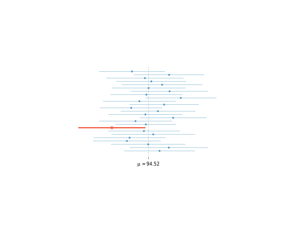
Hence, a confidence interval is not a probability statement about ${\theta}$ .

A 95 percent confidence interval does not mean that the interval would capture the true value 95 percent of the time. This statement would be absurd, because the experiment is conducted after assuming that the ${\theta}$ is a fixed quantity (which is the basic assumption we need while doing frequentist inference).

A sample taken from a population cannot make probability statements about ${\theta}$ , which is the parameter of the probability distribution from which we derived the sample.

The 95 in a 95 percent confidence interval only serves to give us the percentage of time the confidence interval would be right, across trials of all possible experiments, including the ones which are not about this ${\theta}$ parameter that is being discussed.

Confidence Interval Meaning

As an example, on day 1, you collect data and construct a 95 percent confidence interval for a parameter ${\theta_1}$ .

On day 2, you collect new data and construct a 95 percent confidence interval for an unrelated parameter ${\theta_2}$ . On day 3, you collect new data and construct a 95 percent confidence interval for an unrelated parameter ${\theta_3}$ .

You continue this way constructing confidence intervals for a sequence of unrelated parameters ${\theta_1, \theta_2, \dotsc, \theta_n}$ .

Then 95 percent of your intervals will trap the true parameter value.

Hypothesis Testing and p-values

1. Introduction

Hypothesis testing is a method of inference.

Definition 1 A hypothesis is a statement about a population parameter.

Definition 2 Null and Alternate Hypothesis: We partition the parameter space ${\Theta}$ into two disjoint sets ${\Theta_0}$ and ${\Theta_1}$ and we wish to test:

$\displaystyle H_0 \colon \theta \in \Theta_0 \\ H_1 \colon \theta \in \Theta_1. \ \ \ \ \ (1)$

We call ${H_0}$ the null hypothesis and ${H_1}$ the alternate hypothesis.

Definition 3 Rejection Region: Let ${X}$ be a random variable and let ${\mathcal{X}}$ be its range. Let ${R \subset \mathcal{X}}$ be the rejection region.

We accept ${H_0}$ when ${X}$ does not belong to ${R}$ and reject when it does.

Hypothesis testing is a legal trial. We accept ${H_0}$ unless the evidence suggests otherwise. Falsely sentencing the accused when he is not guilty is type I error and letting the accused go free when he is infact guilty is a type II error.

Definition 4 Power Function of a Test: It is the probability of ${X}$ being in the rejection region, expressed as a function of ${\theta}$ .

$\displaystyle \beta(\theta) = \mathbb{P}_{\theta}(X \in R) \ \ \ \ \ (2)$

Definition 5 Size of a Test: It is the maximum of the power function of a test when ${\theta}$ is restricted to the ${\Theta_0}$ parameter space.

$\displaystyle \alpha = \underset{\theta \in \Theta_0}{\text{sup}}(\beta(\theta)). \ \ \ \ \ (3)$

Definition 6 Level ${\alpha}$ Test: A test with size less than or equal to ${\alpha}$ is said to be a level ${\alpha}$ test.

Definition 7 Simple Hypothesis: A hypothesis of the form ${\theta = \theta_0}$ is called a simple hypothesis.

Definition 8 Composite Hypothesis: A hypothesis of the form ${\theta < \theta_0}$ or ${\theta > \theta_0}$ is called a composite hypothesis.

Definition 9 Two Sided Test: A test of the form

$\displaystyle H_0 \colon \theta = \theta_0 \\ H_1 \colon \theta \neq \theta_0. \ \ \ \ \ (4)$

is called a two-sided test.

Definition 10 One Sided Test: A test of the form

$\displaystyle H_0 \colon \theta < \theta_0 \\ H_1 \colon \theta > \theta_0. \ \ \ \ \ (5)$

or

$\displaystyle H_0 \colon \theta > \theta_0 \\ H_1 \colon \theta < \theta_0. \ \ \ \ \ (6)$

is called a one-sided test.

Example 1 (Hypothesis Testing on Normal Distribution:) Let ${X_1, \dotsc, X_n \sim N(\mu, \sigma^2)}$ where ${\sigma}$ is known. We want to test ${H_0 \colon \mu \leq 0}$ versus ${H_1 \colon \mu > 0}$ . Hence ${\Theta_0 = (- \infty, 0]}$ and ${\Theta_1 = ( 0, \infty)}$ .

Consider the test:

$\displaystyle \text{reject } H_0 \text{ if } T > c \ \ \ \ \ (7)$

where ${T = \overline{X}}$ .

Then the rejection region is

$\displaystyle R = \{(x_1, \dotsc, x_n) : \overline{X} > c \} \ \ \ \ \ (8)$

The power function of the test is

$\displaystyle \beta(\mu) = \mathbb{P}_{\mu}(X \in R) \\ = \mathbb{P}_{\mu}(\overline{X} > c) \\ = \mathbb{P}_{\mu}\left( \frac{\sqrt{n}(\overline{X} - \mu)}{\sigma} > \frac{\sqrt{n}(c - \mu)}{\sigma} \right) \\ = \mathbb{P}_{\mu}\left( Z > \frac{\sqrt{n}(c - \mu)}{\sigma} \right) \\ = 1 - \Phi\left(\frac{\sqrt{n}(c - \mu)}{\sigma}\right). \ \ \ \ \ (9)$

The size of the test is

$\displaystyle \text{size} = \underset{\mu \leq 0}{\text{sup}}(\beta(\mu)) \\ = \underset{\mu \leq 0}{\text{sup}}\left(1 - \Phi\left(\frac{\sqrt{n}(c - \mu)}{\sigma}\right)\right) \\ = \beta(0) \\ = 1 - \Phi\left(\frac{c\sqrt{n}}{\sigma}\right). \ \ \ \ \ (10)$

Equating with ${\alpha}$ we obtain

$\displaystyle \alpha = 1 - \Phi\left(\frac{c\sqrt{n}}{\sigma}\right). \ \ \ \ \ (11)$

Hence

$\displaystyle c = \frac{\sigma \thinspace \Phi^{-1}(1 - \alpha)}{\sqrt{n}}. \ \ \ \ \ (12)$

We reject when ${\overline{X} > c}$ . For a test size of 95%

$\displaystyle c = \frac{1.96 \sigma}{\sqrt{n}}. \ \ \ \ \ (13)$

or we reject when

$\displaystyle \overline{X} > \frac{1.96 \sigma}{\sqrt{n}}. \ \ \ \ \ (14)$

2. The Wald Test

Let ${X_1, \dotsc, X_n}$ be \textsc{iid} random variables with ${\theta}$ as a parameter of their distribution function ${F_X(x; \theta)}$ . Let ${\hat{\theta}}$ be the estimate of ${\theta}$ and let ${\widehat{\textsf{se}}}$ be the standard deviation of the distribution of ${\hat{\theta}}$ .

Definition 11 (The Wald Test)

Consider testing a two-sided hypothesis:

$\displaystyle H_0 \colon \theta = \theta_0 \\ H_1 \colon \theta \neq \theta_0. \ \ \ \ \ (15)$

Assume that ${\hat{\theta}}$ has an asymptotically normal distribution.

$\displaystyle \frac{\hat { \theta } - \theta }{\widehat{\textsf{se}} } \rightsquigarrow N(0, 1). \ \ \ \ \ (16)$

Then, the size ${\alpha}$ the Wald Test is: reject ${H_0}$ if ${|W| > z_{\alpha/2}}$ where

$\displaystyle W = \frac{\hat { \theta } - \theta_0 }{\widehat{\textsf{se}}}. \ \ \ \ \ (17)$

Theorem 12 Asymptotically, the Wald test has size ${\alpha}$ .

$\displaystyle size \\ = \underset{\theta \in \Theta_0}{\text{sup}}(\beta(\theta)) \\ = \underset{\theta \in \Theta_0}{\text{sup}}\mathbb{P}_{\theta}(X \in R) \\ = \mathbb{P}_{\theta_0}(X \in R) \\ = \mathbb{P}_{\theta_0}(|W| > z_{\alpha/2}) \\ = \mathbb{P}_{\theta_0}\left(\left| \frac{\hat { \theta } - \theta_0 }{\widehat{\textsf{se}}}\right| > z_{\alpha/2}\right) \\ \rightarrow \mathbb{P}(|Z| > z_{\alpha/2}) \\ = \alpha. \ \ \ \ \ (18)$

Example 2 Two experiments are conducted to test two prediction algorithms.

The prediction algorithms are used to predict the outcomes ${n}$ and ${m}$ times, respectively, and have a probability of predicting with success as ${p_1}$ and ${p_2}$ , respectively.

Let ${\delta = p_1 - p_2}$ .

Consider testing a two-sided hypothesis:

$\displaystyle H_0 \colon \delta = 0 \\ H_1 \colon \delta \neq 0. \ \ \ \ \ (19)$

3. The Likelihood Ratio Test

This test can be used to test vector valued parameters as well.

Definition 13 The likelihood ratio test statistic for testing ${H_0 \colon \theta \in \Theta_0}$ versus ${H_1 \colon \theta \in \Theta_1}$ is

$\displaystyle \lambda(x) = \frac{ \underset{\theta \in \Theta_0}{\text{sup}} (L( \theta|\mathbf{x} )) }{ \underset{\theta \in \Theta}{\text{sup}} (L( \theta|\mathbf{x} )) }. \ \ \ \ \ (20)$

Parametric Inference

There are two methods of estimating ${\theta}$ .

1. Method of Moments

It is a method of generating parametric estimators. These estimators are not optimal but they are easy to compute. They are also used to generate starting values for other numerical parametric estimation methods.

Definition 1 Moments and Sample Moments:

Suppose that the parameter ${\theta}$ has ${k}$ components: ${\theta = (\theta_1,\dotsc,\theta_k)}$ . For ${1 \leq j \leq k}$ ,

Define ${j^{th}}$ moment as

$\displaystyle \alpha_j \equiv \alpha_j(\theta) = \mathbb{E}_\theta(X^j) = \int \mathrm{x}^{j}\,\mathrm{d}F_{\theta}(x). \ \ \ \ \ (1)$

Define ${j^{th}}$ sample moment as

$\displaystyle \hat{\alpha_j} = \frac{1}{n}\sum_{i=1}^n X_i^j. \ \ \ \ \ (2)$

Definition 2

The method of moments estimator ${\hat{\theta_n}}$ is the value of ${\theta}$ which satisfies

$\displaystyle \alpha_1(\hat{\theta_n}) = \hat{\alpha_1} \\ \alpha_2(\hat{\theta_n}) = \hat{\alpha_2} \\ \vdots \vdots \vdots \\ \alpha_k(\hat{\theta_n}) = \hat{\alpha_k} \ \ \ \ \ (3)$

Why The Above Method Works: The method of moments estimator is obtained by equating the ${j^{th}}$ moment with the ${j^{th}}$ sample moment. Since there are k of them we get k equations in k unknowns (the unknowns are the k parameters). This works because we can find out the ${j^{th}}$ moments in terms of the unknown parameters and we can find the ${j^{th}}$ sample moments numerically, since we know the sample values.

2. Maximum Likelihood Method

It is the most common method for estimating parameters in a parametric model.

Definition 3 Likelihood Function: Let ${X_1, \dotsc, X_n}$ have a \textsc{pdf} ${ f_X(x;\theta)}$ . The likelihood function is defined as

$\displaystyle \mathcal{L}_n(\theta) = \prod_{i=1}^n f_X(X_i;\theta). \ \ \ \ \ (4)$

The log-likelihood fucntion is defined as ${\ell_n(\theta) = \log(\mathcal{L}_n(\theta))}$ .

The likelihood function is the joint density of the data. We treat it as a function of the parameter ${\theta}$ . Thus ${\mathcal{L}_n \colon \Theta \rightarrow [0, \infty)}$ .

Definition 4 Maximum Likelihood Estimator: It is the value of ${\theta}$ , ${\hat{\theta}}$ which maximizes the likelihood function.

Example 1 Let ${X_1, \dotsc, X_n}$ be \textsc{iid} random variables with ${\text{Unif}(0, \theta)}$ distribution.

$\displaystyle f_X(x; \theta) = \begin{cases} 1/\theta 0 < x < \theta \\ 0 \text{otherwise}. \end{cases} \ \ \ \ \ (5)$

If ${X_{max} = \max\{X_1, \dotsc, X_n \}}$ and ${X_{max} > \theta}$ , then ${\mathcal{L}_n(\theta) = 0}$ . Otherwise ${\mathcal{L}_n(\theta) = (\frac{1}{\theta})^n }$ which is a decreasing function of ${\theta}$ . Hence ${\hat{\theta} = \max\{ \mathcal{L}_n(\theta)\} = X_{max}}$ .

3. Properties of MLE

Consistent: MLE is consistent: The estimate converges to the true value in probability.

Equivariant: MLE is equivariant. Functions of estimate are estimator of functions of true parameters.

Asymptotically Normal: MLE is asymptotically normal.

Asymptotically Optimal It has the smallest variance among all other well behaved estimators.

Bayes Estimator: MLE is also the Bayes Estimator.

4. Consistency of MLE

Definition 5 Kullback Leibler Distance:
If ${f}$ and ${g}$ are \textsc{pdf}, the Kullback Leibler distance between them is defined as

$\displaystyle D(f, g) = \int f(x) \log \left( \frac{f(x) }{g(x) } \right) dx. \ \ \ \ \ (6)$

5. Equivariance of MLE

6. Asymptotic Normality of MLE

The distribution of ${\hat{\theta}}$ is asymptotically normal. We need the following definitions to prove it.

Definition 6 Score Function: Let ${X}$ be a random variable with \textsc{pdf} ${f_X(x; \theta)}$ . Then the score function is defined as

$\displaystyle s(X; \theta) = \frac{\partial \log f_X(x; \theta) }{\partial \theta}. \ \ \ \ \ (7)$

Definition 7 Fisher Information: The Fisher Information is defined as

$\displaystyle I_n(\theta) = \mathbb{V}_{\theta}\left( \sum_{i=1}^n s(X_i; \theta) \right) \\ = \sum_{i=1}^n \mathbb{V}_{\theta}\left(s(X_i; \theta) \right). \ \ \ \ \ (8)$

Theorem 8

$\displaystyle \mathbb{E}_{\theta}(s(X; \theta)) = 0. \ \ \ \ \ (9)$

Theorem 9

$\displaystyle \mathbb{V}_{\theta}(s(X; \theta)) = \mathbb{E}_{\theta}(s^2(X; \theta)). \ \ \ \ \ (10)$

Theorem 10

$\displaystyle I_n(\theta) = nI(\theta). \ \ \ \ \ (11)$

Theorem 11

$\displaystyle I(\theta) = -\mathbb{E}_{\theta}\left( \frac{\partial^2 \log f_X(x; \theta) }{\partial \theta^2} \right) \\ = -\int \left( \frac{\partial^2 \log f_X(x; \theta) }{\partial \theta^2} \right)f_X(x; \theta) dx. \ \ \ \ \ (12)$

Definition 12 Let ${ \textsf{se} = \sqrt{\mathbb{V}(\hat{\theta} ) } }$ .

Theorem 13

$\displaystyle \textsf{se} \approx \sqrt{1/I_n(\theta)}. \ \ \ \ \ (13)$

Theorem 14

$\displaystyle \frac{\hat { \theta } - \theta }{\textsf{se} } \rightsquigarrow N(0, 1). \ \ \ \ \ (14)$

Theorem 15 Let ${ \hat{\textsf{se}} = \sqrt{1/I_n(\hat{\theta)}} }$ .

$\displaystyle \frac{\hat { \theta } - \theta }{\hat{\textsf{se}}} \rightsquigarrow N(0, 1). \ \ \ \ \ (15)$

In words, ${(a, b)}$ traps ${\theta}$ with probability ${1 - \alpha}$ . We call ${1 - \alpha}$ the coverage of the confidence interval. ${C_n}$ is random and ${\theta}$ is fixed. Commonly, people use 95 percent confidence intervals, which corresponds to choosing ${\alpha}$ = 0.05. If ${\theta}$ is a vector then we use a confidence set (such as a sphere or an ellipse) instead of an interval.

Theorem 16 (Normal Based Confidence Intervals)

Let ${\hat{\theta} \approx N(\theta,\hat{\textsf{se}}^2 )}$ .

and let ${\Phi}$ be the \textsc{cdf} of a random variable ${Z}$ with standard normal distribution and

$\displaystyle z_{\alpha / 2} = \Phi^{- 1 } ( 1 - \alpha / 2) \\ \mathbb{P}(Z > z _{\alpha / 2} ) = ( 1 - \alpha / 2) \\ \mathbb{P}(- z _{\alpha / 2} < Z < z _{\alpha / 2}) = 1 - \alpha. \ \ \ \ \ (16)$

and let

$\displaystyle C_n = \left( \hat{\theta} - z _{\alpha / 2}\hat{\textsf{se}} , \hat{\theta} + z _{\alpha / 2}\hat{\textsf{se}} \right) \ \ \ \ \ (17)$

Then,

$\displaystyle \mathbb{P}_{\theta} (\theta \in C _n ) \rightarrow 1 - \alpha. \ \ \ \ \ (18)$

For 95% confidence intervals ${ 1 - \alpha}$ is .95, ${\alpha}$ is .05, ${z _{\alpha / 2}}$ is 1.96 and the interval is thus ${ C_n = \left( \hat{\theta} - z _{\alpha / 2}\hat{\textsf{se}} , \hat{\theta} + z _{\alpha / 2}\hat{\textsf{se}} \right) = \left( \hat{\theta} - 1.96\hat{\textsf{se}} , \hat{\theta} + 1.96\hat{\textsf{se}} \right) }$ .

Introduction to Statistical Inference

1. Introduction

We assume that the data we are looking at comes from a probability distribution with some unknown parameters that control the exact shape of the distribution.

Definition 1 Statistical Inference: It is the process of using given data to infer the properties of the distribution (for example the values of the parameters) which generated the data. It is also called ‘learning’ in computer science.

Definition 2 Statistical Models: A statistical model is a set of distributions.

When we find out the form of the distribution (the equations that describe it) and the parameters used in the form we gain more understanding of the source of our data.

2. Parametric Models

Definition 3 Parametric Models: A parametric model is a statistical model which is parameterized by a finite number of parameters. A general form of a parametric model is

$\displaystyle \mathfrak{F} = \{f(x;\theta) : \theta \in \Theta\} \ \ \ \ \ (1)$

where ${\theta}$ is an unknown parameter (or vector of parameters) that can take values in the parameter space ${\Theta}$ .

Example 1 An example of a parametric model is:

$\displaystyle \mathfrak{F} = \{f(x;\mu, \sigma) = \frac{1}{\sigma\sqrt{2\pi}}exp\{-\frac{1}{2\sigma^2}(x-\mu)^2\}, \mu \in \mathbb{R}, \sigma > 0\} \ \ \ \ \ (2)$

3. Non-Parametric Models

Definition 4 Non – Parametric Models: A non-parametric model is one in which ${\mathfrak{F}_{ALL} = \{\text{all CDF's}\}}$ cannot be parameterized by a finite number of parameters.

3.1. Non-Paramateric Estimation of Functionals

Definition 5 Sobolev Space: Usually, it is not possible to estimate the probability distribution from the data by just assuming that it exists. We need to restrict the space of possible solutions. One way is to assume that the density function is a smooth function. The restricted space is called Sobolev Space.

Definition 6 Statistical Functional: Any function of \textsc{cdf} ${F}$ is called a statistical functional.

Example 2 Statistical Functionals: The mean, variance and median can be thought of as functions of ${F}$ :

The mean ${\mu}$ is given as:

$\displaystyle \mu = T(F) = \int x dF(x) \ \ \ \ \ (3)$

The variance is given as:

$\displaystyle T(F) = \int x^2 dF(x) - \left(\int xdF(x)\right)^2 \ \ \ \ \ (4)$

The median is given as:

$\displaystyle T(F) = F^{-1}(x) \ \ \ \ \ (5)$

4. Regression

Definition 7 Independent and Dependent Variables: We observe pairs of data: ${(X_1, Y_1),\dotsc,(X_n, Y_n)}$ . ${Y}$ is assumed to depend on ${X}$ which is assumed to be the independent variable. The other names for these are, for:

${X}$ : predictor, regressor, feature or independent variable.
${Y}$ : response variable, outcome or dependent variable.

Definition 8 Regression Function: The regression function is

$\displaystyle r(X) = \mathbb{E}(Y|X=x) \ \ \ \ \ (6)$

Definition 9 Parametric and Non-Parametric Regression Models: If we assume that ${r \in \mathfrak{F} \text{ and } \mathfrak{F}}$ is finite dimensional, then the model is a parametric regression model, otherwise it is a non-parametric regression model.

There can be three categories of regression, based on the purpose for which it was done:

Prediction,
Classification and
Curve Estimation

Definition 10 Prediction: The goal of predicting ${Y}$ based on the value of ${X}$ is called prediction.

Definition 11 Classification: If ${Y}$ is discrete then prediction is instead called classification.

Definition 12 Curve Estimation: If our goal is to estimate the function ${r}$ , then we call this regression or curve estimation.

The regression function ${r(X) = \mathbb{E}(Y|X=x)}$ can be algebraically manipulated to express it in the form

$\displaystyle Y = r(X) + \epsilon \ \ \ \ \ (7)$

where ${\mathbb{E}(\epsilon) = 0}$ .

If ${\mathfrak{F} = \{f(x;\theta) : \theta \in \Theta\}}$ is a parametric model, then we write ${P_{\theta}(X \in A) = \int_A f_X(x) dx }$ to denote the probability that X belongs to A. It does not mean that we are averaging over ${\theta}$ , it means that the probability is calculated assuming the parameter is ${\theta}$ .

5. Fundamental Concepts in Inference

Many inferential problems can be identified as being one of three types: estimation, confidence sets, or hypothesis testing.

5.1. Point Estimates

Definition 13 Point Estimation: Point estimation refers to providing a single “best guess” of some quantity of interest. The quantity of interest could be

a parameter in a parametric model,
a \textsc{cdf} ${F}$ ,
a probability density function ${f}$ ,
a regression function ${r}$ , or
a prediction for a future value ${Y}$ of some random variable.

By convention, we denote a point estimate of ${\theta \text{ by } \hat{\theta}}$ . Since ${\theta}$ is a fixed, unknown quantity, the estimate ${\hat{\theta}}$ depends on the data so ${\hat{\theta}}$ is a random.

Definition 14 Point Estimator of ${\hat{\theta}_n}$ : Formally, let ${X_1, \dotsc, X_n}$ be n \textsc{iid} data points from some distribution ${F}$ . Then, a point estimator ${\hat { \theta } }$ of ${\theta}$ is some function of ${X_1, \dotsc, X_n}$ :

$\displaystyle \hat { \theta } = g( X_1, \dotsc, X_n ). \ \ \ \ \ (8)$

Definition 15 Bias of an Estimator: The bias of an estimator is defined as:

$\displaystyle \textsf{bias}(\hat{\theta}) = \mathbb{E}( \hat{\theta} ) - \theta. \ \ \ \ \ (9)$

Definition 16 Consistent Estimator: A point estimator ${\hat { \theta } }$ of ${\theta}$ is consistent if: ${\hat{\theta} \xrightarrow{P} \theta}$ .

Definition 17 Sampling Distribution: The distribution of ${\hat{\theta}}$ is called sampling distribution.

Definition 18 Standard Error: The standard deviation of the sampling distribution is called standard error denoted by \textsf{se}.

$\displaystyle \textsf{se} = \textsf{se}(\hat{\theta}) = \sqrt{\mathbb{V}(\hat{\theta})}. \ \ \ \ \ (10)$

In some cases, \textsf{se} depends upon the unkown distribution ${F}$ . Its estimate is denoted by ${\widehat{\textsf{se}}}$ .

Definition 19 Mean Squared Error: It is used to evaluate the quality of a point estimator. It is defined as

$\displaystyle \textsf{\textsc{mse}}(\hat{\theta}) = \mathbb{E}_{ \theta } ( \hat{\theta} - \theta)^2. \ \ \ \ \ (11)$

Example 3 Let ${X_1, \dotsc, X_n}$ be \textsc{iid} random variables with Bernoulli distribution. Then ${\hat { p } = \frac{1}{n} \sum_{i = 1}^nX_i }$ . Then, ${\mathbb{E}( \hat { p }) = p}$ . Hence, ${\hat { p }}$ is unbiased.

Definition 20 Asymptotically Normal Estimator: An estimator is asymptotically normal if

$\displaystyle \frac{\hat { \theta } - \theta }{\textsf{se} } \rightsquigarrow N(0, 1). \ \ \ \ \ (12)$

5.2. Confidence Sets

Definition 21 A ${1 - \alpha}$ confidence interval for a parameter ${\theta}$ is an interval ${C_n = (a, b)}$ (where ${a = a(X_1,\dotsc, X_n ) }$ and ${b = b(X_1,\dotsc, X_n ) }$ are functions of the data), such that

$\displaystyle \mathbb{P}_\theta(\theta \in C_n) \geq 1 - \alpha, \forall \: \theta \in \Theta. \ \ \ \ \ (13)$

Theorem 22 (Normal Based Confidence Intervals)

Let ${\hat{\theta} \approx N(\theta,\hat{\textsf{se}}^2 )}$ .

and let ${\Phi}$ be the \textsc{cdf} of a random variable ${Z}$ with standard normal distribution and

$\displaystyle z_{\alpha / 2} = \Phi^{- 1 } ( 1 - \alpha / 2) \\ \mathbb{P}(Z > z _{\alpha / 2} ) = ( 1 - \alpha / 2) \\ \mathbb{P}(- z _{\alpha / 2} < Z < z _{\alpha / 2}) = 1 - \alpha. \ \ \ \ \ (14)$

and let

$\displaystyle C_n = \left( \hat{\theta} - z _{\alpha / 2}\hat{\textsf{se}} , \hat{\theta} + z _{\alpha / 2}\hat{\textsf{se}} \right) \ \ \ \ \ (15)$

Then,

$\displaystyle \mathbb{P}_{\theta} (\theta \in C _n ) \rightarrow 1 - \alpha. \ \ \ \ \ (16)$

5.3. Hypothesis Testing

In hypothesis testing, we start with some default theory – called a null hypothesis – and we ask if the data provide sufficient evidence to reject the theory. If not we retain the null hypothesis.

Convergence of Random Variables

1. Introduction

There are two main ideas in this article.

Law of Large Numbers:
This states that the mean of the sample ${\overline{X}_n}$ converges in probability to the distribution mean ${\mu}$ as ${n}$ increases.

Central Limit Theorem:
This states that the distribution of the sample mean converges in distribution to a normal distribution as ${n}$ increases.

2. Types of Convergence

Let ${X_1, \dotsc, X_n}$ be a sequence of random variables with distributions ${F_n}$ and let ${X}$ be a random variable with distribution ${F}$ .

Definition 1 Convergence in Probability: ${X_n}$ converges to ${X}$ in probability, written as ${X_n \overset{P}{\longrightarrow} X}$ , if for every ${\epsilon > 0}$ , we have

$\displaystyle \mathbb{P}(|X_n - X| > \epsilon) \rightarrow 0 \ \ \ \ \ (1)$

as ${n \rightarrow \infty}$ .

Definition 2 Convergence in Distribution: ${X_n}$ converges to ${X}$ in distribution, written as ${X_n \rightsquigarrow X}$ , if

$\displaystyle \underset{n \rightarrow \infty}{\text{lim}} F_n(t) = F(t) \ \ \ \ \ (2)$

at all ${t}$ for which ${F}$ is continuous.

3. The Law of Large Numbers

Let ${X_1, X_2, \dotsc}$ be \textsc{iid} with mean ${\mu = \mathbb{E}(X_1)}$ and variance ${\sigma^2 = \mathbb{V}(X_1)}$ . Let sample mean be defined as ${\overline{X}_n = (1/n)\sum_{i=1}^n X_i}$ . It can be shown that ${\mathbb{E}(\overline{X}_n) = \mu}$ and ${\mathbb{V}(\overline{X}_n) = \sigma^2/n}$ .

Theorem 3 Weak Law of Large Numbers: If ${X_1, \dotsc, X_n}$ are \textsc{iid} random variables, then ${\overline{X}_n \overset{P}{\longrightarrow} \mu}$ .

4. The Central Limit Theorem

The law of large numbers says that the distribution of the sample mean, ${\overline{X}_n}$ , piles up near the true distribution mean, ${\mu}$ . The central limit theorem further adds that the distribution of the sample mean approaches a Normal distribution as n gets large. It even gives the mean and the variance of the normal distribution.

Theorem 4 The Central Limit Theorem: Let ${X_1, \dotsc, X_n}$ be \textsc{iid} random variables with mean ${\mu}$ and standard deviation ${\sigma}$ . Let sample mean be defined as ${\overline{X}_n = (1/n)\sum_{i=1}^n X_i}$ . Then the asymptotic behaviour of the distribution of the sample mean is given by

$\displaystyle Z_n = \frac{ (\overline{X}_n - \mu) } { \sqrt{ \mathbb{V}( \overline{X}_n ) } } = \frac{ \sqrt{n}(\overline{X}_n - \mu) } { \sigma } \rightsquigarrow N(0,1) \ \ \ \ \ (3)$

The other ways of expressing the above equation are

$\displaystyle Z_n \approx N(0, 1) \\ \overline{X}_n \approx N\left(\mu, \frac{\sigma^2}{n}\right) \\ (\overline{X}_n - \mu) \approx N(0, \sigma^2/n) \\ \sqrt{n}(\overline{X}_n - \mu) \approx N(0,\sigma^2) \\ \frac{\sqrt{n}(\overline{X}_n - \mu)}{\sigma} \approx N(0,1). \ \ \ \ \ (4)$

Definition 5 As has been defined in the Expectation chapter, if ${X_1, \dotsc, X_n}$ are random variables, then we define the sample variance as

$\displaystyle S_n^2 = \frac{1}{n - 1}\left(\sum_{i=1}^n (\overline{X}_n - X_i)^2\right). \ \ \ \ \ (5)$

Theorem 6 Assuming the conditions of the CLT,

$\displaystyle \frac{\sqrt{n}(\overline{X}_n - \mu)}{S_n} \approx N(0,1). \ \ \ \ \ (6)$

5. The Delta Method

Theorem 7 Let ${Y_n}$ be a random variable with conditions of CLT met, and let ${g(x)}$ be a differentiable function with ${g'(\mu) \neq 0}$ . Then,

$\displaystyle Y_n \approx N\left(\mu, \frac{\sigma^2}{n}\right) \\ \Longrightarrow \quad g(Y_n) \approx N\left(g(\mu), (g'(\mu))^2\frac{\sigma^2}{n}\right). \ \ \ \ \ (7)$

Expectation of Random Variables

1. Expectation of a Random Variable

The expectation of a random variable is the average value of ${X}$ .

Definition 1 The expectation, mean or first moment of ${X}$ is defined to be

$\displaystyle \mathbb{E}(X) = \int x f(x) dx = \begin{cases} \sum_x x f(x) X \text{ is discrete} \\ \int_x x f(x) dx X \text{ is continuous}. \end{cases} \ \ \ \ \ (1)$

The following notations are also used.

$\displaystyle \mathbb{E}(X) = \mathbb{E}X = \int x \thinspace dF(x) = \mu_X = \mu \ \ \ \ \ (2)$

Theorem 2 The Rule of the Lazy Statistician: Let ${Y = r(X)}$ , then the expectation of Y is

$\displaystyle \mathbb{E}(Y) = \int r(X) \thinspace dF_X(x). \ \ \ \ \ (3)$

2. Properties of Expectation

Theorem 3 If ${X_1, \dotsc, X_n}$ are random variables and ${a_1, \dotsc, a_n}$ are constants, then

$\displaystyle \mathbb{E}\left(\sum_{i=1}^n a_iX_i\right) = \sum_{i=1}^na_i\mathbb{E}(X_i). \ \ \ \ \ (4)$

Theorem 4 If ${X_1, \dotsc, X_n}$ are independent random variables, then

$\displaystyle \mathbb{E}\left(\prod_{i=1}^n X_i\right) = \prod_{i=1}^n\mathbb{E}(X_i). \ \ \ \ \ (5)$

3. Variance and Covariance

Definition 5 Let ${X}$ be a random variable with mean ${\mu}$ . The variance of ${X}$ , denoted by ${\mathbb{V}(X)}$ , ${\mathbb{V}X}$ , or ${\sigma^2}$ or ${\sigma_X^2}$ is defined by:

$\displaystyle \mathbb{V}(X) = \mathbb{E}((X - \mu)^2) = \int (X - \mu)^2 \thinspace dF(x) \ \ \ \ \ (6)$

assuming the variance exists. The standard deviation is the square root of the variance.

Definition 6 If ${X_1, \dotsc, X_n}$ are random variables, then we define the sample mean as

$\displaystyle \overline{X}_n = \frac{1}{n}\left(\sum_{i=1}^n X_i\right). \ \ \ \ \ (7)$

Definition 7 If ${X_1, \dotsc, X_n}$ are random variables, then we define the sample variance as

$\displaystyle S_n^2 = \frac{1}{n - 1}\left(\sum_{i=1}^n (\overline{X}_n - X_i)^2\right). \ \ \ \ \ (8)$

4. Properties of Variance

Theorem 8

$\displaystyle \mathbb{V}(X) = \mathbb{E}(X^2) - \mu^2. \ \ \ \ \ (9)$

Theorem 9 If ${a}$ and ${b}$ are constants, then

$\displaystyle \mathbb{V}(aX + b) = a^2 \mathbb{V}(X). \ \ \ \ \ (10)$

Theorem 10 If ${X_1, \dotsc, X_n}$ are random variables and ${a_1, \dotsc, a_n}$ are constants, then

$\displaystyle \mathbb{V}\left(\sum_{i=1}^n a_iX_i\right) = \sum_{i=1}^n{a_i}^2\mathbb{V}(X_i). \ \ \ \ \ (11)$

Theorem 11 If ${X_1, \dotsc, X_n}$ are \textsc{iid} random variables with mean ${\mu}$ and variance ${\sigma^2}$ , then

$\displaystyle \mathbb{E}(\overline{X}_n) = \mu, \quad \mathbb{V}(\overline{X}_n) = \frac{\sigma^2}{n} \quad \text{ and } \quad \mathbb{E}(S_n^2) = \sigma^2. \ \ \ \ \ (12)$

Random Variables

1. Introduction

Definition 1

Random Variable: A random variable ${X}$ is a mapping
$\displaystyle X \colon \Omega \rightarrow \mathbb{R} \ \ \ \ \ (1)$

which assigns real numbers ${X(\omega)}$ to outcomes ${\omega}$ in ${\Omega}$ .

2. Distribution Functions

Definition 2

Distribution Function: Given a random variable ${X}$ , the cumulative distribution function (also called the \textsc{cdf}) is a function ${F_X \colon \mathbb{R} \rightarrow [0,1]}$ defined by:
$\displaystyle F_X(x) = \mathbb{P}(X \leq x) \ \ \ \ \ (2)$

Theorem 3 Let ${X}$ have \textsc{cdf} ${F}$ and let ${Y}$ have \textsc{cdf} ${G}$ . If ${F(x) = G(x)}$ for all ${x \in \mathbb{R}}$ then ${\mathbb{P}(X \in A) = \mathbb{P}(Y \in A)}$ for all ${A}$ .

Definition 4 ${X}$ is discrete if it takes countably many infinite values.

We define the probability function or the probability mass function for ${X}$ by ${f_X(x) = \mathbb{P}(X = x)}$ .

Definition 5 A random variable ${X}$ is said to be continuous if there exists a function ${f_X}$ such that

${f_X(x) \geq 0}$ for all ${x \in \mathbb{R}}$ ,
${\int_{-\infty}^{\infty}f_X(x)dx = 1}$
for all ${a, b \in \mathbb{R}}$ with ${a \leq b}$ we have
$\displaystyle \int_a^b f_X(x)dx = \mathbb{P}(a < X < b) \ \ \ \ \ (3)$

The function ${f_X}$ is called the probability density function and we have

$\displaystyle F_X(x) = \int_{-\infty}^x f_X(t)dt \ \ \ \ \ (4)$

and ${f_X(x) = F_X'(X)}$ at all points for which ${F_X}$ is differentiable.

3. Important Discrete Random Variables

Remark 1 We write ${X \sim F}$ to denote that the random variable ${X}$ has a \textsc{cdf} ${F}$ .

3.1. The Point Mass Distribution

\textsc{The Point Mass Distribution}. X has a point mass distribution at ${a}$ , written ${X \sim \delta_a}$ if ${\mathbb{P}(X = a) = 1}$ . Hence ${F_X}$ is

$\displaystyle F_X(x) = \begin{cases} 0& x < a \\ 1& x \geq a. \end{cases} \ \ \ \ \ (5)$

3.2. The Discrete Uniform Distribution

\textsc{The Discrete Uniform Distribution}. Let ${k > 1}$ be a given integer. Let ${X}$ have a probability mass function given by:

$\displaystyle f_X(x) = \begin{cases} 1/k & 1 \leq x \leq k \\ 0 & \text{otherwise}. \end{cases} \ \ \ \ \ (6)$

Then ${X}$ has a discrete uniform distribution on ${{1, \dotsc , k}}$ .

3.3. The Bernoulli Distribution

\textsc{The Bernoulli Distribution}. Let ${X}$ be a random variable with ${\mathbb{P}(X = 1) = p}$ and ${\mathbb{P}(X = 0) = 1 - p}$ for some ${p \in [0, 1]}$ . We say that ${X}$ has a Bernoulli Distribution written as ${X \sim \text{Bernoulli}(p)}$ . The probability function ${f_X}$ is given by ${f_X(x) = p^x(1 - p)^{(1 - x)} \text{ for } x \in {0, 1}}$ .

3.4. The Binomial Distribution

\textsc{The Binomial Distribution}. Flip a coin ${n}$ times and let ${X}$ denote the number of heads. If ${p}$ denotes the probability of getting heads in a single coin toss and the tosses are assumed to be independent then the \textsc{pdf} of ${X}$ can be shown to be:

$\displaystyle f_X(x) = \begin{cases} \begin{pmatrix} n \\ x \end{pmatrix} p^x(1 - p)^{(n-x)} & 0 \leq x \leq n \\ 0 & \text{otherwise}. \end{cases} \ \ \ \ \ (7)$

3.5. The Geometric Distribution

\textsc{The Geometric Distribution}. ${X}$ has a geometric distribution with parameter ${p \in [0, 1]}$ , written as ${X \sim \text{Geom}(p)}$ if

$\displaystyle f_X(x) = p(1 - p)^{(x - 1)} \text{ for } x \in \{1, 2, 3, \dotsc , \}. \ \ \ \ \ (8)$

${X}$ is the number of flips needed until the first head appears.

3.6. The Poisson Distribution

\textsc{The Poisson Distribution}. ${X}$ has a Poisson distribution with parameter ${\lambda > 0}$ , written as ${X \sim \text{Poisson}(\lambda)}$ if

$\displaystyle f_X(x) = e^{-\lambda}\frac{\lambda^{-x}}{x!} \text{ for } x \geq 0. \ \ \ \ \ (9)$

${X}$ is the probability of a given number of events occurring in a fixed interval of time and/or space if these events occur with a known average rate and independently of the time since the last event.

4. Important Continuous Random Variables

4.1. The Uniform Distribution

\textsc{The Uniform Distribution}. For ${a, b \in \mathbb{R} \text{ and } a < b}$ , X has a uniform distribution over ${(a, b)}$ , written ${X \sim \text{Uniform}(a, b)}$ , if

$\displaystyle f_X(x) = \begin{cases} \frac{1}{b - a} & x \in [a, b] \\ 0 & \text{otherwise}. \end{cases} \ \ \ \ \ (10)$

4.2. The Normal Distribution

\textsc{The Normal Distribution}. We say that ${X}$ has a normal (or Gaussian) distribution with parameters ${\mu}$ and ${\sigma}$ , written as ${X \sim N(\mu, \sigma^2)}$ if

$\displaystyle f_X(x;\mu, \sigma) = \frac{1}{\sigma\sqrt{2\pi}}exp\left\{-\frac{1}{2\sigma^2}(x-\mu)^2\right\}, \text{ where } \mu, \sigma \in \mathbb{R}, \sigma > 0. \ \ \ \ \ (11)$

The parameter ${\mu}$ is the “center” (or mean) of the distribution and ${\sigma}$ is the “spread” (or standard deviation) of the distribution. We say that ${X}$ has a standard Normal distribution if ${\mu = 0}$ and ${\sigma = 1}$ . A standard Normal random variable is denoted by ${Z}$ . The \textsc{pdf} and \textsc{cdf} of a standard Normal are denoted by ${\phi(z)}$ and ${\Phi(z)}$ . The \textsc{pdf} is plotted in Figure There is no closed-form expression for ${\Phi}$ . Here are some useful facts:

If ${X \sim N(\mu, \sigma^2)}$ , then ${Z = (X - \mu) / \sigma \sim N(0, 1)}$ .

If ${Z \sim N(0, 1)}$ , then ${X = \mu + \sigma Z \sim N(\mu, \sigma^2)}$ .

If ${X_i \sim N(\mu_i, \sigma_i^2)}$ for ${i = 1, \dotsc , n}$ are independent, then we have

$\displaystyle \sum_{i = 1}^nX_i \sim N\left(\sum_{i=1}^n \mu_i, \sum_{i=1}^n \sigma_i^2\right). \ \ \ \ \ (12)$

It follows from ${(i)}$ that if ${X \sim N(\mu, \sigma^2)}$

$\displaystyle \mathbb{P}\left(a < X < b\right) \ \ \ \ \ (13)$

$\displaystyle \mathbb{P}\left(a < X < b\right) = \mathbb{P}\left(a < \mu + \sigma Z < b\right) \ \ \ \ \ (14)$

$\displaystyle \mathbb{P}\left(a < X < b\right) = \mathbb{P}\left(\frac{a - \mu}{\sigma} < Z < \frac{b - \mu}{\sigma}\right) \ \ \ \ \ (15)$

$\displaystyle \mathbb{P}\left(a < X < b\right) = \Phi\left(\frac{b - \mu}{\sigma}\right) - \Phi\left(\frac{a - \mu}{\sigma}\right). \ \ \ \ \ (16)$

Example 1 Suppose that ${X \sim N(3, 5)}$ . Find ${P(X > 1)}$ .

Solution:

$\displaystyle \mathbb{P}\left(X > 1\right) \\ = \mathbb{P}\left(3 + Z\sqrt{5} > 1\right) \\ = \mathbb{P}\left( Z > \frac{-2}{\sqrt{5}}\right) \\ = 1 - \Phi\left(\frac{2}{\sqrt{5}}\right) \\ = 1 - \Phi\left(0.894427\right) \\ = 0.81. \ \ \ \ \ (17)$

Example 2 For the above problem, also find the value ${x}$ of ${X}$ such that ${\mathbb{P}(X < x) = .2}$ . Solution:

$\displaystyle 0.2 = \mathbb{P}\left(X < x\right) \\ = \mathbb{P}\left(3 + Z\sqrt{5} < x\right) \\ = \mathbb{P}\left(Z < \frac{x - 3}{\sqrt{5}}\right) \\ = \Phi\left(\frac{x - 3}{\sqrt{5}}\right) \ \ \ \ \ (18)$

From the normal table, we have that ${\Phi(-0.8416) = 0.2}$

$\displaystyle \Phi(-0.8416) = \Phi\left(\frac{x - 3}{\sqrt{5}}\right) \\ -0.8416 = \left(\frac{x - 3}{\sqrt{5}}\right) \\ x = \left(3 - 0.8416\times\sqrt{5}\right) \\ x = 1.1181. \ \ \ \ \ (19)$

4.3. The Exponential Distribution

\textsc{The Exponential Distribution}. ${X}$ has an exponential distribution with parameter ${\beta > 0}$ , written as ${X \sim \text{Exp}(\beta)}$ , if

$\displaystyle f_X(x) = \frac{1}{\beta}e^{-x/\beta}, \text{ for } x > 0. \ \ \ \ \ (20)$

4.4. The Gamma Distribution

\textsc{The Gamma Distribution}. For ${\alpha > 0}$ , the Gamma function is defined as

$\displaystyle \Gamma(\alpha) = \int_0^\infty y^{\alpha - 1} e^{-y} dy. \ \ \ \ \ (21)$

${X}$ has a Gamma distribution with parameters ${\alpha}$ and ${\beta}$ (where ${\alpha, \beta > 0}$ ), written as ${X \sim \text{Gamma}(\alpha, \beta)}$ , if

$\displaystyle f_X(x) = \frac{1}{\beta^{\alpha}\Gamma(\alpha)}x^{\alpha - 1}e^{-x/\beta}, \text{ for } x > 0. \ \ \ \ \ (22)$

5. Bivariate Distributions

Definition 6 Given a pair of discrete random variables ${X}$ and ${Y}$ , their joint mass function is defined as ${f_{X, Y}(x,y) = \mathbb{P}(X = x, Y = y)}$

Definition 7 For two continuous random variables, ${X}$ and ${Y}$ , we call a function ${f_{X,Y}}$ a \textsc{pdf} of random variables ${(X, Y)}$ if

${f_{X, Y}(x, y) \geq 0}$ for all ${(x, y) \in \mathbb{R}^2}$ ,
${\int_{-\infty}^{\infty}\int_{-\infty}^{\infty}f_{X,Y}(x, y) \thinspace dx \thinspace dy = 1}$
For any set ${A \in \mathbb{R}^2}$ we have
$\displaystyle \int \int_A f_{X,Y}(x, y) \thinspace dx \thinspace dy = \mathbb{P}((X,Y) \in A). \ \ \ \ \ (23)$

Example 3 For ${-1 \leq x \leq 1}$ , let ${(X, Y)}$ have density

$\displaystyle f_{X, Y}(x,y) = \begin{cases} cx^2y x^2 \leq y \leq 1, \\ 0 \text{otherwise}. \end{cases} \ \ \ \ \ (24)$

Find the value of ${c}$ .

Solution: We equate the integral of ${f}$ over ${\mathbb{R}^2}$ to ${1}$ and find ${c}$ .

$\displaystyle 1 = \int_{-\infty}^{\infty}\int_{-\infty}^{\infty}f_{X,Y}(x, y) \thinspace dy \thinspace dx \\ = \int_{-1}^{1}\int_{x^2}^{1}f_{X,Y}(x, y) \thinspace dy \thinspace dx \\ = \int_{-1}^{1}\int_{x^2}^{1}cyx^2 \thinspace dy \thinspace dx \\ = \int_{-1}^{1}c\left(\frac{1 - x^4}{2}\right)x^2 \thinspace dx \\ = \left(\frac{c}{2}\right)\left(\int_{-1}^{1}x^2 \thinspace dx - \int_{-1}^{1}x^6 \thinspace dx \right)\\ = \left(\frac{c}{2}\right)\left( \frac{2}{3} - \frac{2}{7}\right)\\ = \left(\frac{4c}{21}\right) \\ c = \frac{21}{4} \ \ \ \ \ (25)$

6. Marginal Distributions

Definition 8 For the discrete case, if ${X, Y}$ have a joint mass distribution ${f_{X, Y}}$ then the marginal distribution of ${X}$ is given by

$\displaystyle f_X(x) = \mathbb{P}(X = x) = \sum_y \mathbb{P}(X = x, Y = y) = \sum_y f_{X,Y}(x, y) \ \ \ \ \ (26)$

and of ${Y}$ is given by

$\displaystyle f_Y(y) = \mathbb{P}(Y = y) = \sum_x \mathbb{P}(X = x, Y = y) = \sum_x f_{X,Y}(x, y) \ \ \ \ \ (27)$

Definition 9 For the continuous case, if ${X, Y}$ have a probability distribution function ${f_{X, Y}}$ then the marginal distribution of ${X}$ is given by

$\displaystyle f_X(x) = \int f_{X,Y}(x, y) \thinspace dy \ \ \ \ \ (28)$

and of ${Y}$ is given by

$\displaystyle f_Y(y) = \int f_{X,Y}(x, y) \thinspace dx \ \ \ \ \ (29)$

7. Independent Random Variables

Definition 10 Two random variables, ${X}$ and ${Y}$ are said to be independent if for every ${A}$ and ${B}$ we have

$\displaystyle \mathbb{P}(X \in A, Y \in B) = \mathbb{P}(X \in A)\mathbb{P}(Y \in B) \ \ \ \ \ (30)$

Theorem 11 Let ${X}$ and ${Y}$ have a joint \textsc{pdf} ${f_{X, Y}}$ . Then ${X \amalg Y}$ if ${f_{X, Y}(x, y) = f_X(x)f_Y(y)}$ for all values of ${x}$ and ${y}$ .

8. Conditional Distributions

Definition 12 Let ${X}$ and ${Y}$ have a joint \textsc{pdf} ${f_{X, Y}}$ . Then the conditional distribution of ${X}$ given Y is defined as

$\displaystyle f_{X|Y}(x|y) = \frac{f_{X, Y}(x, y)}{f_Y(y)} \ \ \ \ \ (31)$

9. Multivariate Distributions and \textsc

Samples}

Definition 13 Independence of ${n}$ random variables: Let ${X = \begin{pmatrix} X_1, \dotsc, X_n \end{pmatrix}}$ where ${X_1, \dotsc, X_n}$ are random variables. Let ${f(x_1, x_2, \dotsc, x_n)}$ denote their \textsc{pdf}. We say that ${X_1, \dotsc, X_n}$ are independent if for every ${A_1, \dotsc, A_n}$ ,

$\displaystyle \mathbb{P}(X_1 \in A_1, \dotsc, X_n \in A_n) = \prod_{i=1}^n \mathbb{P}(X_i \in A_i) \ \ \ \ \ (32)$

Definition 14 If ${X_1, \dotsc, X_n}$ are independent random variables with the same marginal distribution ${F}$ , we say that ${X_1, \dotsc, X_n}$ are \textsc{iid} (identically and independently distributed) random variables and we write:

$\displaystyle \begin{pmatrix} X_1, \dotsc, X_n \end{pmatrix} \sim F \ \ \ \ \ (33)$

If ${F}$ has density ${f}$ then we also write ${\begin{pmatrix} X_1, \dotsc, X_n \end{pmatrix} \sim f}$ . We also call ${X_1, \dotsc, X_n}$ a random sample of size ${n}$ from ${F}$ .

10. The Multivariate Normal Distribution

\textsc{The Multivariate Normal Distribution} In the multivariate normal distribution, the parameter ${\mu}$ is a vector and the parameter ${\sigma}$ is a matrix ${\Sigma}$ . Let

$\displaystyle Z = \begin{pmatrix} Z_1 \\ \vdots \\ Z_k \end{pmatrix} \ \ \ \ \ (34)$

where ${Z_1, \dotsc, Z_k \sim N(0, 1)}$ are independent. The joint density of ${Z}$ is

$\displaystyle f_Z(z) = \frac{1}{{(2\pi)}^{k/2}}\text{exp}\biggl\{-\frac{1}{2}\sum_{j=1}^k {z_j}^2\biggr\} = \frac{1}{{(2\pi)}^{k/2}}\text{exp}\left\{-\frac{1}{2}z^Tz\right\} \\ f_X(x;\mu, \Sigma) = \frac{1}{{(2\pi)}^{k/2}{|\Sigma |}^{1/2}}\text{exp}\left\{-\frac{1}{2}(x - \mu)^T\Sigma^{-1}(x - \mu)\right\} \ \ \ \ \ (35)$

Frequentists and Bayesians

1. Interpretations of Probability

1.1. Bayesians and Frequentists

There are two possible ways to interpret the meaning of probability.

1.2. Maps and Territories

Here ‘territory’ refers to the world as it exists or the reality as it is.

The map refers to our model of the world or the way we see and interpret it.

We are constantly building ‘maps’ or models of the territory. The better our maps the closer we are to the ‘truth’.

1.3. PDFs – Existence in Maps or Territory

The main contention between frequentists and bayesians is the question: “Where do probability density functions exist – Do they exist in the map or in the territory?”

Frequentists hold that the probability density functions exist in the territory.

Bayesians believe that they exist only in our map of reality.

For example, suppose we toss a coin. Then the frequentists believe that there is a probability density function which is independent of our maps and interpretation of reality which forms the basis of randomness that is observed in the coin toss. Bayesians believe that if we know the force applied the fingers tossing the coin, the mass, shape and the orientation of the coin, the movement of molecules in the air at the time of tossing it, in summary if we have a very accurate model of reality than the probability density function changes and it might come to a point in this case where the entire question of coins landing heads or tails may become deterministic.

1.4. Many Worlds Interpretation of Quantum Mechanics

This states that there are multiple universe and each one corresponds to some combination of values which the various probability distributions of position and momentum happen to generate. If the many worlds interpretation is correct then our world is deterministic. Then the probability can only be in the map and not the territory.

Probability

1. Introduction

Probability is the mathematical language for quantifying uncertainty.

2. Sample Space and Events

The setup begins with an experiment being conducted. It can have a number of outcomes. The following are then defined:

Definition 1

Sample Space: The sample space ${\Omega}$ is the set of all possible outcomes.

Definition 2

Realizations, Sample Outcomes or Elements: These refer to points ${\omega}$ in ${\Omega}$ .

Definition 3

Events: Subsets of sample space are called events.

Example 1 If we toss a coin twice then ${\Omega = \lbrace HT, TH, HH, TT\rbrace}$ and the event that the first toss is heads is ${A = \lbrace HH, HT\rbrace}$ .

The complements, unions, intersections and differences of event sets can be defined and interpreted trivially. ${\Omega}$ is the true event and ${\emptyset}$ is the false event.

Definition 4

Disjoint or Mutually Exclusive Events: ${A_1, A_2, \dotsc,}$ are mutually exclusive events if ${A_i \bigcap A_j = \emptyset}$ whenever ${i \neq j}$ .

Definition 5

Partition of ${\Omega}$ : A partition of ${\Omega}$ is a sequence of disjoint sets such that their union is ${\Omega}$ .

3. Probability

Definition 7

Probability Distribution or a Probability Measure: A function ${\mathbb{P}}$ is called a probability measure or a probability distribution if it satisfies the following three axioms:
Axiom 1: ${\mathbb{P}(\Omega) = 1}$ .
Axiom 2: ${\mathbb{P}(A) \geq 0}$ for every ${A}$ .
Axiom 3: If ${A_1, A_2, \dotsc, }$ are disjoint, then:
$\displaystyle \mathbb{P}\left(\bigcup \limits_{i=1}^{\infty} A_i\right) = \sum_{i=1}^{\infty}\mathbb{P}(A_i) \ \ \ \ \ (2)$

4. Properties of Probability Distributions

One can derive many properties from the definition of probability distribution (Definition 7).

$\displaystyle \mathbb{P}(\emptyset) = 0 \ \ \ \ \ (3)$

$\displaystyle A \subset B \Longrightarrow \mathbb{P}(A) \leq \mathbb{P}(B) \ \ \ \ \ (4)$

$\displaystyle 0 \leq \mathbb{P}(A) \leq 1 \ \ \ \ \ (5)$

$\displaystyle \mathbb{P}(A^c) = 1 - \mathbb{P}(A) \ \ \ \ \ (6)$

$\displaystyle A \bigcap B = \emptyset \Longrightarrow \mathbb{P}\left(A \bigcup B\right) = \mathbb{P}(A) + \mathbb{P}(B) \ \ \ \ \ (7)$

Lemma 8 If ${A}$ and ${B}$ are two events, then

$\displaystyle \mathbb{P}\left(A \bigcup B\right) = \mathbb{P}(A) + \mathbb{P}(B) - \mathbb{P}\left(A \bigcap B\right) \ \ \ \ \ (8)$

Theorem 9 Continuity of Probabilities: If ${A_n \rightarrow A}$ , then

$\displaystyle \mathbb{P}(A_n) \rightarrow \mathbb{P}(A) \ \ \ \ \ (9)$

as ${n \rightarrow \infty}$ .

5. Probability on Finite Sample Spaces

If the sample space ${\Omega = \{\omega_1, \omega_2, \dotsc, \omega_n\}}$ is finite and each outcome is equally likely, then:

$\displaystyle \mathbb{P}(A) = \frac{|A|}{|\Omega|} \ \ \ \ \ (10)$

Given ${n}$ objects, the number of ways of arranging or permuting them is

$\displaystyle n! = 1 \times 2 \times \dotsb \times (n - 1) \times n \ \ \ \ \ (11)$

Given ${n}$ objects, the number of ways of selecting or choosing ${k \text{ (where } 1 \leq k \leq n)}$ out of them is

$\displaystyle \begin{pmatrix} n \\ k \end{pmatrix} = \frac{n!}{k!(n-k)!} \ \ \ \ \ (12)$

For example, the number of ways to chose 3 students out of a class of 20 is

$\displaystyle \begin{pmatrix} 20 \\ 3 \end{pmatrix} = \frac{20!}{3!(17)!} = \frac{20 \times 19 \times 18}{1 \times 2 \times 3} = 1140 \ \ \ \ \ (13)$

6. Independent Events

Definition 10

Independent Events: Two events, ${A}$ and ${B}$ are said to be independent if
$\displaystyle \mathbb{P}(AB) = \mathbb{P}(A)\mathbb{P}(B) \ \ \ \ \ (14)$

A set of events ${\{A_i : i \in I\} }$ is independent if

$\displaystyle \mathbb{P}\left(\bigcap_{i \in J} A_i\right) = \prod_{i \in J} \left(\mathbb{P}(A_i)\right) \ \ \ \ \ (15)$

for every finite subset ${J}$ of ${I}$ .

Independence can be of two types – assumed or derived.

Two disjoint events cannot be independent.

7. Conditional Probability

Definition 11

Conditional Probability: The conditional probability of ${A}$ given ${B}$ has occurred is
$\displaystyle \mathbb{P}(A|B) = \frac{\mathbb{P}(A \bigcap B)}{\mathbb{P}(B)}. \ \ \ \ \ (16)$

Remark 1 ${\mathbb{P}(A|B)}$ is the fraction of times ${A}$ occurs in cases when ${B}$ has occurred.

Lemma 12 If ${A}$ and ${B}$ are independent events then ${\mathbb{P}(A|B) = \mathbb{P}(A)}$ . Also, for any pair of events ${A}$ and ${B}$

$\displaystyle \mathbb{P}(AB) = \mathbb{P}(A|B)\mathbb{P}(B) = \mathbb{P}(B|A)\mathbb{P}(A). \ \ \ \ \ (17)$

8. Bayes’ Theorem

Theorem 13

The Law of Total Probability: Let ${A_1, A_2, \dotsc, A_n}$ be a partition of ${\Omega}$ and let ${B}$ be any event, then:
$\displaystyle \mathbb{P}(B) = \sum_{i=1}^n \mathbb{P}(B|A_i)\mathbb{P}(A_i). \ \ \ \ \ (18)$

Overview of Total Probability Theorem:

We are given
- a partition of the sample space and
- any other event B.
We have found a relation between
- the probability of the single event B and
- the probabilities of the events comprising the partition and the conditional probabilities of the single event B given the events in the partition.

Theorem 14

Bayes’ Theorem: Let ${A_1, A_2, \dotsc, A_n}$ be a partition of ${\Omega}$ such that ${\mathbb{P}(A_i) > 0 }$ for each ${i}$ . If ${\mathbb{P}(B) > 0}$ , then for each ${i = 1, \dotsc, n}$ :
$\displaystyle \mathbb{P}(A_i|B) = \frac{\mathbb{P}(B|A_i)\mathbb{P}(A_i)}{\sum_{j=1}^n \mathbb{P}(B|A_j)\mathbb{P}(A_j)}. \ \ \ \ \ (19)$

Overview of Bayes’ Theorem:

Inputs: We are given

A partition of the sample space: A set of n events covering the sample space.

An other event ${B}$ : ${B}$ is not part of the partition.

Relation Found: We have found a relation between

Probability of ${A_i|B}$ : The probability of the partition events given the single event ${B}$ has occurred.

This has been expressed in terms of

Probability of ${B|A_i}$ : The probability of the single event ${B}$ given the partition events have occurred.

Example 2 Suppose that ${A_1, A_2 \text{ and } A_3}$ are the events that an email is spam, low priority or high priority, respectively. Let ${\mathbb{P}(A_1) = .7, \thinspace \mathbb{P}(A_2) = .2, \text{ and } \mathbb{P}(A_3) = .1 }$ .

Let ${B}$ be the event that the email contains the word “free”.

Let ${\mathbb{P}(B|A_1) = .9, \thinspace \mathbb{P}(B|A_2) = .02, \text{ and } \mathbb{P}(B|A_3) = .01 }$ .

If the email received has the word “free”, what is the probability that it is spam?

Here,

$\displaystyle \mathbb{P}(Spam Email | Email has Word Free) = \mathbb{P}(A_1|B) \ \ \ \ \ (20)$

$\displaystyle \mathbb{P}(A_1|B) = \frac{\mathbb{P}(B|A_1)\mathbb{P}(A_1)}{\sum_{j=1}^3 \mathbb{P}(B|A_j)\mathbb{P}(A_j)} = \frac{.9 \times .7}{.9 \times .7 + .01 \times .2 + .01 \times .1} = .995. \ \ \ \ \ (21)$