Statistics – Gaurav Sharma's Blog

In the following codes an attempt is made to raise the abstraction level available to the sas programmer by providing list manipulation macros:

Markov Model for Loss Forecasting – Implementation in SAS

Here’s the sas code that implements the markov model for loss forecasting:

The Need For MapReduce and NoSQL

The Need for MapReduce

Relational Database Management Systems have been in use since 1970s. They provide the SQL language interface.

They are good at needle in the haystack problems – finding small results from big datasets.

They provide a number of advantages:

A declarative query language
Schemas
Logical Data Independence
Database Indexing
Optimizations Through Use of Relational Algebra
Views
Acid Properties (Atomicity, Consistency, Isolation and Durability)

They provide scalability in the sense that even if the data doesn’t fit in main memory, the query will finish efficiently.

However, they are not good at scalability in another sense – that is, having multiple machines available, or multi-cores available will not reduce the time the query takes.

The need thus arose for a system which gives scalability when more machines are added and is thus able to process huge datasets (in 50 GB or more range).

The NoSQL databases give up on atleast one of the ACID properties to achieve better performance on parallel and/or distributed hardware.

Introduction to Hadoop

Apache Hadoop is a software framework for distributed processing of very large datasets.

It provides a distributed storage system Hadoop Distributed File System (HDFS)), and a processing part of the system MapReduce.

The system is so designed so as to recover from hardware failures in some nodes that make up the distributed cluster.

Hadoop is itself written in Java. There are interfaces to use the framework from other languages.

Files on hadoop system are stored in a distributed manner. They are split into blocks which are then stored on different nodes.

The map and reduce functions that a user of hadoop framework writes are packaged and sent to different nodes where they are processed in parallel.

Architecture

The Hadoop framework is composed of the following four modules:

Hadoop Common: – The libraries needed by the other Hadoop modules;
Hadoop Distributed File System (HDFS): A distributed file-system that stores data on commodity machines.
Hadoop YARN: A platform responsible for managing computing resources in clusters.
Hadoop MapReduce: A programming model for large scale data processing.

HDFS

Files in HDFS are broken into blocks. The default block size is 64MB.

An HDFS cluster has two types of nodes – namenode (it works as the master node) and a number of datanodes (these work as the worker nodes).

The namenodes manages the filesystem namespace, maintains the filesystem tree, and the metadata of each file.

The user does not directly have to interact with the namenode or datanodes. A client does that on the user’s behalf. The client also provides a POSIX like filesystem interface.

MapReduce Engine

The MapReduce Engine sits on top of the HDFS filesystem. It consists of one JobTracker and a TaskTracker. The MapReduce jobs of the client applications are submitted to the JobTracker, which pushes the work to the available TaskTracker nodes in the cluster.

The filesystem is designed such that the JobTracker can know the nodes that contain the data, and how far they are.

The TaskTracker communicates with the JobTracker every few minutes to check its status.

The Job Tracker and TaskTracker expose their status and information through Jetty. This can be viewed from a web browser.

By default Hadoop uses FIFO scheduling. The job scheduler in modern versions is separate and it is possible to use an alternate scheduler (eg. Fair scheduler , Capacity scheduler).

The Hadoop Ecosystem

The term “Hadoop” now refers not just to the 4 base modules above, but also to the ecosystem, or collection of additional software packages that can be installed on top of or alongside Hadoop.

Examples of these are

Impala,

Apache Sqoop,

Difference Equations

1. Difference Equations

1.1. Introduction

Time series analysis deals with a series of random variables.

1.2. First Order Difference Equations

We will study time indexed random variables ${y_t}$ .

Let ${y_t}$ be a linear function of ${y_{t-1}}$ and ${w_t}$ .

$\displaystyle y_t = \phi{y_t} + w_t \ \ \ \ \ (1)$

Equation 1 is a linear first-order difference equation. It is a first-order difference equation because ${y_t}$ only depends on ${y_{t-1}}$ and not on other previous ${y_t}$ s.

In this chapter, we treat ${w_t}$ as a deterministic number and later on we will analyse the effects of treating it as a random variable.

1.3. Solution by Recursive Substitution

The equations are:

$\displaystyle \begin{array}{rcl} y_0 = \phi{y_{-1}} + w_t \\ y_1 = \phi{y_0} + w_t \\ \vdots \\ y_{t-1} = \phi{y_{t-2}} + w_{t-1} \\ y_t = \phi{y_t} + w_t \end{array}$

By recursively substituting we obtain:

$\displaystyle y_t = \phi^{t+1}y_{-1} + \phi^tw_1 + \phi^{t-2}w_2 + \dotsc + \phi{w_{t-1}} + w_t \ \ \ \ \ (2)$

1.4. Dynamic Multipliers

We want to know the effect of increasing ${w_t}$ on ${y_{t+j}}$ . This can be obtained by differentiating equation 10 with respect to ${w_t}$ .

$\displaystyle \frac{\partial y_{t+j}}{\partial w_t} = \phi^{j} \ \ \ \ \ (3)$

2. pth-Order Difference Equations

We generalize the above dynamic system to let the value of y to depend on p of its own lags in addition to the current value of the input variable ${w_t}$ .

$\displaystyle y_t = \phi_{1}y_{-1} + \phi^tw_1 + \phi^{t-2}w_2 + \dotsc + \phi{w_{t-1}} + w_t \ \ \ \ \ (4)$

We will rewrite the above p-th order equation to a vector first order equation.

We define,

$\displaystyle \xi_t= \begin{bmatrix} y_t \\ y_{t - 1} \\ \vdots \\ y_{t - p + 1} \end{bmatrix},\quad \ \ \ \ \ (5)$

$\displaystyle F = \begin{bmatrix} \phi_{1} & \phi_{2} & \phi_{3} & \cdots & \phi_{p - 1} & \phi_{p} \\ 1 & 0 & 0 & \cdots & 0 & 0\\ 0 & 1 & 0 & \cdots & 0 & 0\\ \vdots & \vdots & \vdots & \cdots & \vdots & \vdots \\ 0 & 0 & 0 & \cdots & 0 & 0 \end{bmatrix},\quad \ \ \ \ \ (6)$

$\displaystyle v_t= \begin{bmatrix} w_t \\ 0 \\ 0 \\ \vdots \\ 0 \end{bmatrix},\quad \ \ \ \ \ (7)$

Then,

$\displaystyle \xi_t = F\xi_{t-1} + v_t \ \ \ \ \ (8)$

or,

$\displaystyle \begin{bmatrix} y_t \\ y_{t - 1} \\ y_{t - 3;} \\ \vdots \\ y_{t - p + 1} \end{bmatrix}\quad = \quad \begin{bmatrix} \phi_{1} & \phi_{2} & \phi_{3} & \cdots & \phi_{p - 1} & \phi_{p} \\ 1 & 0 & 0 & \cdots & 0 & 0\\ 0 & 1 & 0 & \cdots & 0 & 0\\ \vdots & \vdots & \vdots & \cdots & \vdots & \vdots \\ 0 & 0 & 0 & \cdots & 0 & 0 \end{bmatrix}\quad \begin{bmatrix} y_{t - 1} \\ y_{t - 2} \\ y_{t - 3} \\ \vdots \\ y_{t - p} \end{bmatrix}\quad + \quad \begin{bmatrix} w_t \\ 0 \\ 0 \\ \vdots \\ 0 \end{bmatrix}\quad \ \ \ \ \ (9)$

Following the approach taken for solving first order difference equation and applying it to the vector equation, we get,

$\displaystyle \xi_t = F^{t+1}\xi_{-1} + F^tv_0 + F^{t-1}v_1 + F^{t-2}v_2 + \dotsc + F{v_{t-1}} + v_t \ \ \ \ \ (10)$

3. General Solution of a p-th Order Difference Equation

If the eigenvalues of F matrix are distinct then we can write F as

$\displaystyle F = T\Lambda T^{-1} \ \ \ \ \ (11)$

$\displaystyle \Lambda = \begin{bmatrix} \lambda_{1} & 0 & 0 & \cdots & 0 \\ 0 & \lambda_{2} & 0 & \cdots & 0 \\ 0 & 0 & \lambda_{3} & \cdots & 0 \\ \vdots & \vdots & \vdots & \cdots & \vdots \\ 0 & 0 & 0 & \cdots & \lambda_{p} \end{bmatrix},\quad \ \ \ \ \ (12)$

where T is a non-singular matrix.

Thus,

$\displaystyle F^2 = T\Lambda^2 T^{-1} \ \ \ \ \ (13)$

and

$\displaystyle \Lambda^2 = \begin{bmatrix} \lambda_{1}^2 & 0 & 0 & \cdots & 0 \\ 0 & \lambda_{2}^2 & 0 & \cdots & 0 \\ 0 & 0 & \lambda_{3}^2 & \cdots & 0 \\ \vdots & \vdots & \vdots & \cdots & \vdots \\ 0 & 0 & 0 & \cdots & \lambda_{p}^2 \end{bmatrix},\quad \ \ \ \ \ (14)$

In general,

$\displaystyle F^n = T\Lambda^n T^{-1} \ \ \ \ \ (15)$

and

$\displaystyle \Lambda^n = \begin{bmatrix} \lambda_{1}^n & 0 & 0 & \cdots & 0 \\ 0 & \lambda_{2}^n & 0 & \cdots & 0 \\ 0 & 0 & \lambda_{3}^n & \cdots & 0 \\ \vdots & \vdots & \vdots & \cdots & \vdots \\ 0 & 0 & 0 & \cdots & \lambda_{p}^n \end{bmatrix},\quad \ \ \ \ \ (16)$

Misconceptions About P Values and The History of Hypothesis Testing

1. Introduction

The misconceptions surrounding p values are an example where knowing the history of the field and the mathematical and philosophical principles behind it can greatly help in understanding.

The classical statistical testing of today is a hybrid of the approaches taken by R. A. Fisher on the one hand and Jerzy Neyman and Egon Pearson on the other.

P-value is often confused with the Type I error rate – ${\alpha}$ of the Neyman-Pearson approach.

In statistics journals and research, the Neyman-Pearson approach replaced the significance testing paradigm 60 years ago, but in empirical work the Fisher approach is pervasive.

The statistical testing approach found in the textbooks on statistics is a hybrid

2. Fisher’s Significance Testing

Fisher held the belief that statistics could be used for inductive inference, that “it is possible to argue from consequences to causes, from observations to hypothesis” and that it it possible to draw inferences from the particular to the general.

Hence he rejected the methods in which probability of a hypothesis given the data, ${\mathop{\mathbb P}(H \vert x)}$ , are used in favour of ones in which probability of data, ${\mathop{\mathbb P}(H \vert x)}$ , given a particular hypothesis are used.

In his approach, the discrepancies in the data are used to reject the null hypothesis. This is done as follows:

The researcher sets up a null hypothesis, which is the status quo belief.

The sampling distribution under the null hypothesis is known.

If the observed data deviates from the mean of the sampling distribution by more than a specified level, called the level of significance, then we reject the null hypothesis. Otherwise, we “fail to reject” the null hypothesis.

The p-value in this approach is the probability of observing data at least as favorable to the alternative hypothesis as our current data set, if the null hypothesis is true.

There is a common misconception that if ${p = .05}$ , then the null hypothesis has only a 5% chance of being true.

This is clearly false, and can be seen from the definition as the P value is calculated under the assumption that the null hypothesis is true. It therefore cannot be a probability of the null hypothesis being false.

Conversely, a p value being high merely means that a null effect is statistically consistent with the observed results.

It does not mean that the null hypothesis is true. We only fail to reject, if we adopt the data based inductive approach.

We need to consider the Type I and Type II error probabilities to draw such conclusions, which is done in the Neyman-Pearson approach.

3. Neyman-Pearson Theory

The main contribution of Neyman-Pearson hypothesis testing framework (they named it to distinguish it from the inductive approach of Fisher’s significance testing) is the introduction of the

probabilities of committing two kinds of errors, false rejection (Type I error), called ${\alpha}$ , and false acceptance (Type II error), called ${\beta}$ , of the null hypothesis.
power of a statistical test. It is defined as the probability of rejecting a false null hypothesis. It is equal to ${1 - \beta}$ .

Fisher’s theory relied on the rejection of null hypothesis based on the data, assuming null hypothesis to be true. In contrast, the Neyman-Pearson approach provides rules to make decisions to choose the between the two hypothesis.

Neyman–Pearson theory, then, replaces the idea of inductive reasoning with that of, what they called, inductive behavior.

In his own words, inductive behaviour was meant to imply: “The term ‘inductive behavior’ means simply the habit of humans and other animals (Pavlov’s dog, etc.) to adjust their actions to noticed frequencies of events, so as to avoid undesirable consequences”.

Then, in this approach, the costs associated with Type I and Type II behaviour determine the decision to accpet or reject. These costs vary from experiment to experiment and this thus is the main advantage of the Neyman-Pearson approach over Fisher’s approach.

Thus while designing the experiment the researcher has to control the probabilities of Type I and Type II errors. The best test is the one that minimizes the Type II error given an upper bound on the Type I error.

And what adds to the source of confusion is the fact that Neyman called the Type I error the level of significance, a term that Fisher used to denote the p values.

Ordinary Least Squares Under Standard Assumptions

Suppose that a scalar ${y_t}$ is related to a ${(k \times 1)}$ vector, ${x_t}$ and a disturbance term ${u_t}$ according to the regression model.

$\displaystyle y_t = x_t^T \beta + u_t \ \ \ \ \ (1)$

In this article, we will study the estimation and hypothesis testing of ${\beta}$ when ${x_t}$ is deterministic and ${u_t}$ is i.i.d. Gaussian.

1. The Algebra of Linear Regression

Given a sample of T values of ${y_t}$ and the vector ${x_t}$ , the ordinary least squares (OLS) estimate of ${\beta}$ , denoted as ${b}$ , is the value of ${\beta}$ which minimizes the residual sum of squares (RSS).

$\displaystyle RSS = \sum_{t=1}^T (y_t - x_t^T b)^2 \ \ \ \ \ (2)$

The OLS estimate of ${\beta}$ , b, is given by:

$\displaystyle b = \bigg(\frac{1}{T}\sum_{t=1}^T x_tx_t^T \bigg)^{\!-1} \!\!\cdot\, \frac{1}{T}\sum_{t=1}^n x_ty_t. \ \ \ \ \ (3)$

The model is written in matrix notation as:

$\displaystyle y = X\beta + u. \ \ \ \ \ (4)$

$\displaystyle \bold{y}= \begin{bmatrix} y_1 \\ y_2 \\ \vdots \\ y_T \end{bmatrix},\quad \bold{x}= \begin{bmatrix} x_1^T \\ x_2^T \\ \vdots \\ x_T^T \end{bmatrix},\quad \bold{u}= \begin{bmatrix} u_1 \\ u_2 \\ \vdots \\ u_T \end{bmatrix}. \ \ \ \ \ (5)$

where ${y}$ is a ${T \times 1}$ vector, ${X}$ is a ${T \times k}$ matrix, ${\beta}$ is a ${k \times 1}$ vector and ${u}$ is a ${T \times 1}$ vector.

Thus,

$\displaystyle b = (X^TX)^{-1}X^Ty. \ \ \ \ \ (6)$

Similarly,

$\displaystyle \hat u = y - Xb = y - X(X^TX)^{-1}X^Ty = [I_T - X(X^TX)^{-1}X^T]y = M_Xy. \ \ \ \ \ (7)$

where ${M_X}$ is defined as:

$\displaystyle M_X = [I_T - X(X^TX)^{-1}X^T]. \ \ \ \ \ (8)$

${M_X}$ is a projection matrix. Hence it is symmetric and idempotent.

$\displaystyle M_X = M_X^T. \ \ \ \ \ (9)$

$\displaystyle M_XM_X = M_X. \ \ \ \ \ (10)$

Since ${M_X}$ is the projection matrix for the space orthogonal to ${X}$ ,

$\displaystyle M_X^TX = M_XX = 0. \ \ \ \ \ (11)$

Thus, we can verify that the sample residuals are orthogonal to ${X}$ .

$\displaystyle u^TX = y^TM_X^TX = 0. \ \ \ \ \ (12)$

The sample residual is constructed from the sample estimate of ${\beta}$ which is ${b}$ . The population residual is a hypothetical construct based on the true population value of ${\beta}$ .

$\displaystyle u_t = y_t - x_t^T \beta. \ \ \ \ \ (13)$

$\displaystyle \hat u_t = y_t - x_t^T b. \ \ \ \ \ (14)$

$\displaystyle \hat u = y - Xb = [I_T - X(X^TX)^{-1}X^T]y = M_Xy = M_XX b + u. \ \ \ \ \ (15)$

$\displaystyle b = (X^TX)^{-1}X^Ty = (X^TX)^{-1}X^T(X\beta + u) = \beta + (X^TX)^{-1}X^Tu. \ \ \ \ \ (16)$

The fit of OLS is described in terms of ${R_u^2}$ , which is defined as the ratio of squares of the fitted values ( ${x_t^Tb)}$ to the observed values of ${y}$ .

$\displaystyle R_u^2 = \frac{\sum_{t=1}^T b^Tx_tx_t^Tb}{\sum_{t=1}^T y_t^2} = \frac{b^TX^TXb}{y^Ty}. \ \ \ \ \ (17)$

2. Assumptions on X and u

We shall assume that

(a) X will be deterministic

(b) ${u_t}$ is i.i.d with mean 0 and variance ${\sigma^2}$ .

2.1. Properties of Estimated b Under Above Assumptions

Since,

$\displaystyle b = (X^TX)^{-1}X^Ty = (X^TX)^{-1}X^T(X\beta + u) = \beta + (X^TX)^{-1}X^Tu. \ \ \ \ \ (18)$

Taking expectations of both sides, we have,

$\displaystyle \mathop{\mathbb E}(b) = \beta + (X^TX)^{-1}X^T\mathop{\mathbb E}(u) = \beta. \ \ \ \ \ (19)$

And the variance covariance matrix is given by,

$\displaystyle \mathop{\mathbb E}[(b - \beta)(b - \beta)^T] = \mathop{\mathbb E}[((X^TX)^{-1}X^Tu)((X^TX)^{-1}X^Tu)^T] = \sigma^2(X^TX)^{-1}. \ \ \ \ \ (20)$

Thus b is unbiased and is a linear function of y.

2.2. Distribution of Estimated b Under Above Assumptions

As u is Gaussian,

$\displaystyle b = \beta + (X^TX)^{-1}X^Tu. \ \ \ \ \ (21)$

implies that b is also Gaussian.

$\displaystyle b \sim N(\beta, \sigma^2(X^TX)^{-1}). \ \ \ \ \ (22)$

2.3. Properties of Estimated Sample Variance Under Above Assumptions

The OLS estimate of variance of u, ${\sigma^2}$ is given by:

$\displaystyle s^2 = RSS / (T - k) = {\hat u}^T\hat u / (T - k) = u^TM_X^TM_Xu / (T - k) = u^TM_Xu / (T - k). \ \ \ \ \ (23)$

Since ${M_X}$ is a projection matrix and is symmetric and idempotent, it can be written as:

$\displaystyle M_X = P\Lambda P^T. \ \ \ \ \ (24)$

where

$\displaystyle P P^T = I_T. \ \ \ \ \ (25)$

and ${\Lambda}$ is a diagonal matrix with eigenvalues of ${M_X}$ on the diagonal.

Since,

$\displaystyle M_XX = 0. \ \ \ \ \ (26)$

that is, since the two spaces that they represent are orthogonal to each other, it follows that:

$\displaystyle M_Xv = 0. \ \ \ \ \ (27)$

whenever v is a column of X. Since we assume X to be of full rank, there are k such vectors and their eigenvalue is the right hand side, which is 0.

Also since

$\displaystyle M_X = I_T - X(X^TX)^{-1}X^T. \ \ \ \ \ (28)$

Thus, it follows that

$\displaystyle M_Xv = v. \ \ \ \ \ (29)$

whenever v is orthogonal to X. Since there are (T – k) such vectors, ${M_X}$ has (T – k) eigenvectors with eigenvalue 1.

Thus ${\Lambda}$ has k zeroes and (T – k) 1s on the diagonal.

$\displaystyle u^TM_Xu = u^TP\Lambda P^Tu. \ \ \ \ \ (30)$

Let

$\displaystyle w = P^Tu \ \ \ \ \ (31)$

Then,

$\displaystyle u^TM_Xu = u^TP\Lambda P^Tu = w^T\Lambda w = w_1^2 \lambda_1 + w_2^2 \lambda_2 + \dots + w_T^2 \lambda_T. \ \ \ \ \ (32)$

$\displaystyle u^TM_Xu = w_1^2 \lambda_1 + w_2^2 \lambda_2 + \dots + w_{T - k}^2 \lambda_{T - k}. \ \ \ \ \ (33)$

As these ${\lambda}$ s are all unity, we have:

$\displaystyle u^TM_Xu = w_1^2 + w_2^2 + \dots + w_{T - k}^2 . \ \ \ \ \ (34)$

Also,

$\displaystyle \mathop{\mathbb E}(w^Tw) = \mathop{\mathbb E}(P^Tu u^T P) = \sigma^2I_T. \ \ \ \ \ (35)$

Thus, elements of w are uncorrelated with each other, have mean 0 and variance ${\sigma^2}$ .

Since each w has expectation of ${\sigma^2}$ ,

$\displaystyle \mathop{\mathbb E}(u^TM_Xu) = (T - k)\sigma^2. \ \ \ \ \ (36)$

Hence,

$\displaystyle \mathop{\mathbb E}(s^2) = \sigma^2. \ \ \ \ \ (37)$

2.4. Distribution of Estimated Sample Variance Under Above Assumptions

Since

$\displaystyle w = P^Tu \ \ \ \ \ (38)$

when u is Gaussian, w is also Gaussian.

Then,

$\displaystyle u^TM_Xu = w_1^2 \lambda_1 + w_2^2 \lambda_2 + \dots + w_{T - k}^2 \lambda_{T - k}. \ \ \ \ \ (39)$

implies that ${u^TM_Xu}$ is the sum of squares of (T – k) independent ${N(0, \sigma^2)}$ random variables.

Thus,

$\displaystyle RSS^2 / \sigma^2 = u^TM_Xu / \sigma^2 \sim \chi^2 ( T - k). \ \ \ \ \ (40)$

Also, b and ${\hat u}$ are uncorrelated, since,

$\displaystyle \mathop{\mathbb E}[\hat u(b - \beta)^T] = \mathop{\mathbb E}[M_Xu u^T X (X^TX)^{-1} = 0. \ \ \ \ \ (41)$

Since b and ${\hat u}$ are independent, b and ${s^2}$ are also independent.

2.5. t Tests about ${\beta}$ Under Above Assumptions

We wish to test the hypothesis that the ith element of ${\beta}$ , ${\beta_i}$ , is some particular value ${\beta_i^0}$ .

The t-statistic for testing this null hypothesis is

$\displaystyle t = \frac{b_i - \beta_i^0}{\hat \sigma_{b_i}} = \frac{b_i - \beta_i^0}{s (\xi^{ii})^2} \ \ \ \ \ (42)$

where ${ \xi^{ii}}$ denotes the ith column and ith row element of ${(X^TX)^{-1}}$ and ${\hat \sigma_{b_i}}$ is the standard error of the OLS estimate of the ith coefficient.

Under the null hypothesis,

$\displaystyle b_i \sim N(\beta_i^0, \sigma^2 \xi^{ii}). \ \ \ \ \ (43)$

Thus,

$\displaystyle \frac{b_i - \beta_i^0}{\sqrt{\sigma^2 \xi^{ii}}} \sim N(0, 1). \ \ \ \ \ (44)$

Thus,

$\displaystyle t = \frac{{(b_i - \beta_i^0)} / {\sqrt{\sigma^2 \xi^{ii}}}}{\sqrt{s^2 / \sigma^2 }} \ \ \ \ \ (45)$

Thus the numerator is N(0, 1) and the denominator is the square root of a chi-square distribution with (T – k) degrees of freedom. This gives a t-distribution to the variable on the left side.

2.6. F Tests about ${\beta}$ Under Above Assumptions

To generalize what we did for t tests, consider that we have a matrix ${R}$ that represents the restrictions we want to impose on ${\beta}$ , that is ${R\beta}$ gives a vector of the hypothesis that we want to test. Thus,

$\displaystyle H_0 \colon R\beta = r \ \ \ \ \ (46)$

Since,

$\displaystyle b \sim N(\beta, \sigma^2(X^TX)^{-1}). \ \ \ \ \ (47)$

Thus, under ${H_0}$ ,

$\displaystyle Rb \sim N(r, \sigma^2R(X^TX)^{-1}R^T). \ \ \ \ \ (48)$

Theorem 1 If ${z}$ is a ${(n \times 1)}$ vector with ${z \sim N(0, \Sigma^2)}$ and non singular ${\Sigma}$ , then ${z^T\Sigma^{-1} z \sim \chi^2(n)}$ .

Applying the above theorem to the ${Rb - r}$ vector, we have,

$\displaystyle (Rb - r)^T (\sigma^2R(X^TX)^{-1}R^T)^{-1}(Rb - r) \sim \chi^2 (m). \ \ \ \ \ (49)$

Now consider,

$\displaystyle F = (Rb - r)^T (s^2R(X^TX)^{-1}R^T)^{-1}(Rb - r) / m. \ \ \ \ \ (50)$

where sigma has been replaced with the sample estimate s.

Thus,

$\displaystyle F = \frac{[(Rb - r)^T (\sigma^2R(X^TX)^{-1}R^T)^{-1}(Rb - r)] / m}{[RSS / (T - k)]/ \sigma^2} \ \ \ \ \ (51)$

In the above, the numerator is a ${\chi^2(m)}$ distribution divided by its degree of freedom and the denominator is a ${\chi^2(T - k)}$ distribution divided by its degree of freedom. Since b and ${\hat u}$ are independent, the numerator and denominator are also independent of each other.

Hence, the variable on the left hand side has an exact ${F(m , T - k)}$ distribution under ${H_0}$ .

Confidence Interval Interpretation

In frequentist statistics (which is one the used by journals and academia), ${\theta}$ is a fixed quantity, not a random variable.

Hence, a confidence interval is not a probability statement about ${\theta}$ .

A 95 percent confidence interval does not mean that the interval would capture the true value 95 percent of the time. This statement would be absurd, because the experiment is conducted after assuming that the ${\theta}$ is a fixed quantity (which is the basic assumption we need while doing frequentist inference).

A sample taken from a population cannot make probability statements about ${\theta}$ , which is the parameter of the probability distribution from which we derived the sample.

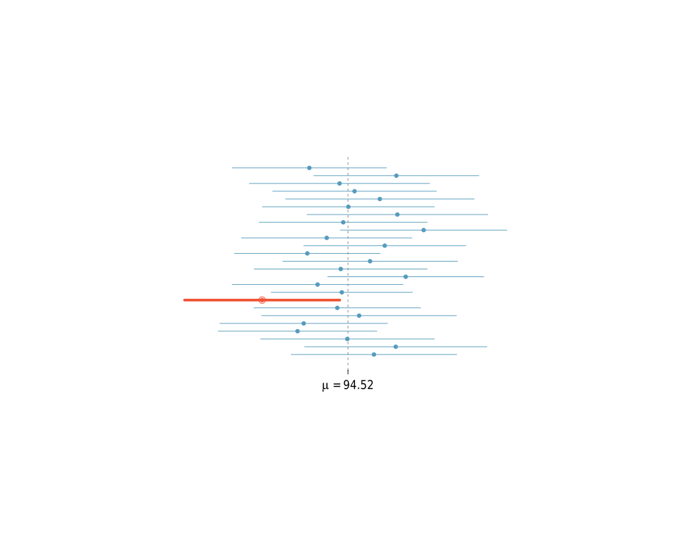
The 95 in a 95 percent confidence interval only serves to give us the percentage of time the confidence interval would be right, across trials of all possible experiments, including the ones which are not about this ${\theta}$ parameter that is being discussed.

Confidence Interval Meaning

As an example, on day 1, you collect data and construct a 95 percent confidence interval for a parameter ${\theta_1}$ .

On day 2, you collect new data and construct a 95 percent confidence interval for an unrelated parameter ${\theta_2}$ . On day 3, you collect new data and construct a 95 percent confidence interval for an unrelated parameter ${\theta_3}$ .

You continue this way constructing confidence intervals for a sequence of unrelated parameters ${\theta_1, \theta_2, \dotsc, \theta_n}$ .

Then 95 percent of your intervals will trap the true parameter value.

Category: Statistics

Protected: Pairwise Classifier

Protected: Fisher Discriminant

Raising Abstraction Level in SAS

Markov Model for Loss Forecasting – Implementation in SAS

The Need For MapReduce and NoSQL

The Need for MapReduce

Introduction to Hadoop

Architecture

HDFS

MapReduce Engine

The Hadoop Ecosystem

Difference Equations

Misconceptions About P Values and The History of Hypothesis Testing

Ordinary Least Squares Under Standard Assumptions

Confidence Interval Interpretation