Inference – Gaurav Sharma's Blog

Misconceptions About P Values and The History of Hypothesis Testing

1. Introduction

The misconceptions surrounding p values are an example where knowing the history of the field and the mathematical and philosophical principles behind it can greatly help in understanding.

The classical statistical testing of today is a hybrid of the approaches taken by R. A. Fisher on the one hand and Jerzy Neyman and Egon Pearson on the other.

P-value is often confused with the Type I error rate – ${\alpha}$ of the Neyman-Pearson approach.

In statistics journals and research, the Neyman-Pearson approach replaced the significance testing paradigm 60 years ago, but in empirical work the Fisher approach is pervasive.

The statistical testing approach found in the textbooks on statistics is a hybrid

2. Fisher’s Significance Testing

Fisher held the belief that statistics could be used for inductive inference, that “it is possible to argue from consequences to causes, from observations to hypothesis” and that it it possible to draw inferences from the particular to the general.

Hence he rejected the methods in which probability of a hypothesis given the data, ${\mathop{\mathbb P}(H \vert x)}$ , are used in favour of ones in which probability of data, ${\mathop{\mathbb P}(H \vert x)}$ , given a particular hypothesis are used.

In his approach, the discrepancies in the data are used to reject the null hypothesis. This is done as follows:

The researcher sets up a null hypothesis, which is the status quo belief.

The sampling distribution under the null hypothesis is known.

If the observed data deviates from the mean of the sampling distribution by more than a specified level, called the level of significance, then we reject the null hypothesis. Otherwise, we “fail to reject” the null hypothesis.

The p-value in this approach is the probability of observing data at least as favorable to the alternative hypothesis as our current data set, if the null hypothesis is true.

There is a common misconception that if ${p = .05}$ , then the null hypothesis has only a 5% chance of being true.

This is clearly false, and can be seen from the definition as the P value is calculated under the assumption that the null hypothesis is true. It therefore cannot be a probability of the null hypothesis being false.

Conversely, a p value being high merely means that a null effect is statistically consistent with the observed results.

It does not mean that the null hypothesis is true. We only fail to reject, if we adopt the data based inductive approach.

We need to consider the Type I and Type II error probabilities to draw such conclusions, which is done in the Neyman-Pearson approach.

3. Neyman-Pearson Theory

The main contribution of Neyman-Pearson hypothesis testing framework (they named it to distinguish it from the inductive approach of Fisher’s significance testing) is the introduction of the

probabilities of committing two kinds of errors, false rejection (Type I error), called ${\alpha}$ , and false acceptance (Type II error), called ${\beta}$ , of the null hypothesis.
power of a statistical test. It is defined as the probability of rejecting a false null hypothesis. It is equal to ${1 - \beta}$ .

Fisher’s theory relied on the rejection of null hypothesis based on the data, assuming null hypothesis to be true. In contrast, the Neyman-Pearson approach provides rules to make decisions to choose the between the two hypothesis.

Neyman–Pearson theory, then, replaces the idea of inductive reasoning with that of, what they called, inductive behavior.

In his own words, inductive behaviour was meant to imply: “The term ‘inductive behavior’ means simply the habit of humans and other animals (Pavlov’s dog, etc.) to adjust their actions to noticed frequencies of events, so as to avoid undesirable consequences”.

Then, in this approach, the costs associated with Type I and Type II behaviour determine the decision to accpet or reject. These costs vary from experiment to experiment and this thus is the main advantage of the Neyman-Pearson approach over Fisher’s approach.

Thus while designing the experiment the researcher has to control the probabilities of Type I and Type II errors. The best test is the one that minimizes the Type II error given an upper bound on the Type I error.

And what adds to the source of confusion is the fact that Neyman called the Type I error the level of significance, a term that Fisher used to denote the p values.

Confidence Interval Interpretation

In frequentist statistics (which is one the used by journals and academia), ${\theta}$ is a fixed quantity, not a random variable.

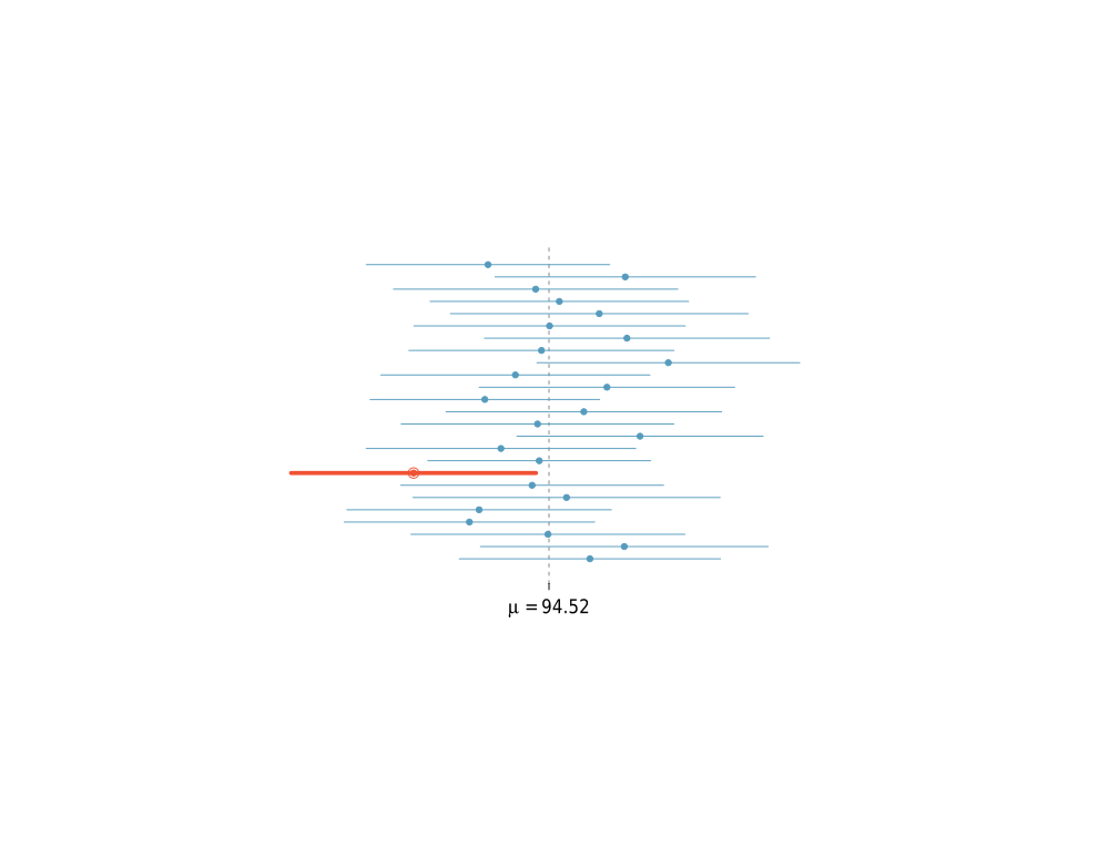
Hence, a confidence interval is not a probability statement about ${\theta}$ .

A 95 percent confidence interval does not mean that the interval would capture the true value 95 percent of the time. This statement would be absurd, because the experiment is conducted after assuming that the ${\theta}$ is a fixed quantity (which is the basic assumption we need while doing frequentist inference).

A sample taken from a population cannot make probability statements about ${\theta}$ , which is the parameter of the probability distribution from which we derived the sample.

The 95 in a 95 percent confidence interval only serves to give us the percentage of time the confidence interval would be right, across trials of all possible experiments, including the ones which are not about this ${\theta}$ parameter that is being discussed.

Confidence Interval Meaning

As an example, on day 1, you collect data and construct a 95 percent confidence interval for a parameter ${\theta_1}$ .

On day 2, you collect new data and construct a 95 percent confidence interval for an unrelated parameter ${\theta_2}$ . On day 3, you collect new data and construct a 95 percent confidence interval for an unrelated parameter ${\theta_3}$ .

You continue this way constructing confidence intervals for a sequence of unrelated parameters ${\theta_1, \theta_2, \dotsc, \theta_n}$ .

Then 95 percent of your intervals will trap the true parameter value.

Hypothesis Testing and p-values

1. Introduction

Hypothesis testing is a method of inference.

Definition 1 A hypothesis is a statement about a population parameter.

Definition 2 Null and Alternate Hypothesis: We partition the parameter space ${\Theta}$ into two disjoint sets ${\Theta_0}$ and ${\Theta_1}$ and we wish to test:

$\displaystyle H_0 \colon \theta \in \Theta_0 \\ H_1 \colon \theta \in \Theta_1. \ \ \ \ \ (1)$

We call ${H_0}$ the null hypothesis and ${H_1}$ the alternate hypothesis.

Definition 3 Rejection Region: Let ${X}$ be a random variable and let ${\mathcal{X}}$ be its range. Let ${R \subset \mathcal{X}}$ be the rejection region.

We accept ${H_0}$ when ${X}$ does not belong to ${R}$ and reject when it does.

Hypothesis testing is a legal trial. We accept ${H_0}$ unless the evidence suggests otherwise. Falsely sentencing the accused when he is not guilty is type I error and letting the accused go free when he is infact guilty is a type II error.

Definition 4 Power Function of a Test: It is the probability of ${X}$ being in the rejection region, expressed as a function of ${\theta}$ .

$\displaystyle \beta(\theta) = \mathbb{P}_{\theta}(X \in R) \ \ \ \ \ (2)$

Definition 5 Size of a Test: It is the maximum of the power function of a test when ${\theta}$ is restricted to the ${\Theta_0}$ parameter space.

$\displaystyle \alpha = \underset{\theta \in \Theta_0}{\text{sup}}(\beta(\theta)). \ \ \ \ \ (3)$

Definition 6 Level ${\alpha}$ Test: A test with size less than or equal to ${\alpha}$ is said to be a level ${\alpha}$ test.

Definition 7 Simple Hypothesis: A hypothesis of the form ${\theta = \theta_0}$ is called a simple hypothesis.

Definition 8 Composite Hypothesis: A hypothesis of the form ${\theta < \theta_0}$ or ${\theta > \theta_0}$ is called a composite hypothesis.

Definition 9 Two Sided Test: A test of the form

$\displaystyle H_0 \colon \theta = \theta_0 \\ H_1 \colon \theta \neq \theta_0. \ \ \ \ \ (4)$

is called a two-sided test.

Definition 10 One Sided Test: A test of the form

$\displaystyle H_0 \colon \theta < \theta_0 \\ H_1 \colon \theta > \theta_0. \ \ \ \ \ (5)$

or

$\displaystyle H_0 \colon \theta > \theta_0 \\ H_1 \colon \theta < \theta_0. \ \ \ \ \ (6)$

is called a one-sided test.

Example 1 (Hypothesis Testing on Normal Distribution:) Let ${X_1, \dotsc, X_n \sim N(\mu, \sigma^2)}$ where ${\sigma}$ is known. We want to test ${H_0 \colon \mu \leq 0}$ versus ${H_1 \colon \mu > 0}$ . Hence ${\Theta_0 = (- \infty, 0]}$ and ${\Theta_1 = ( 0, \infty)}$ .

Consider the test:

$\displaystyle \text{reject } H_0 \text{ if } T > c \ \ \ \ \ (7)$

where ${T = \overline{X}}$ .

Then the rejection region is

$\displaystyle R = \{(x_1, \dotsc, x_n) : \overline{X} > c \} \ \ \ \ \ (8)$

The power function of the test is

$\displaystyle \beta(\mu) = \mathbb{P}_{\mu}(X \in R) \\ = \mathbb{P}_{\mu}(\overline{X} > c) \\ = \mathbb{P}_{\mu}\left( \frac{\sqrt{n}(\overline{X} - \mu)}{\sigma} > \frac{\sqrt{n}(c - \mu)}{\sigma} \right) \\ = \mathbb{P}_{\mu}\left( Z > \frac{\sqrt{n}(c - \mu)}{\sigma} \right) \\ = 1 - \Phi\left(\frac{\sqrt{n}(c - \mu)}{\sigma}\right). \ \ \ \ \ (9)$

The size of the test is

$\displaystyle \text{size} = \underset{\mu \leq 0}{\text{sup}}(\beta(\mu)) \\ = \underset{\mu \leq 0}{\text{sup}}\left(1 - \Phi\left(\frac{\sqrt{n}(c - \mu)}{\sigma}\right)\right) \\ = \beta(0) \\ = 1 - \Phi\left(\frac{c\sqrt{n}}{\sigma}\right). \ \ \ \ \ (10)$

Equating with ${\alpha}$ we obtain

$\displaystyle \alpha = 1 - \Phi\left(\frac{c\sqrt{n}}{\sigma}\right). \ \ \ \ \ (11)$

Hence

$\displaystyle c = \frac{\sigma \thinspace \Phi^{-1}(1 - \alpha)}{\sqrt{n}}. \ \ \ \ \ (12)$

We reject when ${\overline{X} > c}$ . For a test size of 95%

$\displaystyle c = \frac{1.96 \sigma}{\sqrt{n}}. \ \ \ \ \ (13)$

or we reject when

$\displaystyle \overline{X} > \frac{1.96 \sigma}{\sqrt{n}}. \ \ \ \ \ (14)$

2. The Wald Test

Let ${X_1, \dotsc, X_n}$ be \textsc{iid} random variables with ${\theta}$ as a parameter of their distribution function ${F_X(x; \theta)}$ . Let ${\hat{\theta}}$ be the estimate of ${\theta}$ and let ${\widehat{\textsf{se}}}$ be the standard deviation of the distribution of ${\hat{\theta}}$ .

Definition 11 (The Wald Test)

Consider testing a two-sided hypothesis:

$\displaystyle H_0 \colon \theta = \theta_0 \\ H_1 \colon \theta \neq \theta_0. \ \ \ \ \ (15)$

Assume that ${\hat{\theta}}$ has an asymptotically normal distribution.

$\displaystyle \frac{\hat { \theta } - \theta }{\widehat{\textsf{se}} } \rightsquigarrow N(0, 1). \ \ \ \ \ (16)$

Then, the size ${\alpha}$ the Wald Test is: reject ${H_0}$ if ${|W| > z_{\alpha/2}}$ where

$\displaystyle W = \frac{\hat { \theta } - \theta_0 }{\widehat{\textsf{se}}}. \ \ \ \ \ (17)$

Theorem 12 Asymptotically, the Wald test has size ${\alpha}$ .

$\displaystyle size \\ = \underset{\theta \in \Theta_0}{\text{sup}}(\beta(\theta)) \\ = \underset{\theta \in \Theta_0}{\text{sup}}\mathbb{P}_{\theta}(X \in R) \\ = \mathbb{P}_{\theta_0}(X \in R) \\ = \mathbb{P}_{\theta_0}(|W| > z_{\alpha/2}) \\ = \mathbb{P}_{\theta_0}\left(\left| \frac{\hat { \theta } - \theta_0 }{\widehat{\textsf{se}}}\right| > z_{\alpha/2}\right) \\ \rightarrow \mathbb{P}(|Z| > z_{\alpha/2}) \\ = \alpha. \ \ \ \ \ (18)$

Example 2 Two experiments are conducted to test two prediction algorithms.

The prediction algorithms are used to predict the outcomes ${n}$ and ${m}$ times, respectively, and have a probability of predicting with success as ${p_1}$ and ${p_2}$ , respectively.

Let ${\delta = p_1 - p_2}$ .

Consider testing a two-sided hypothesis:

$\displaystyle H_0 \colon \delta = 0 \\ H_1 \colon \delta \neq 0. \ \ \ \ \ (19)$

3. The Likelihood Ratio Test

This test can be used to test vector valued parameters as well.

Definition 13 The likelihood ratio test statistic for testing ${H_0 \colon \theta \in \Theta_0}$ versus ${H_1 \colon \theta \in \Theta_1}$ is

$\displaystyle \lambda(x) = \frac{ \underset{\theta \in \Theta_0}{\text{sup}} (L( \theta|\mathbf{x} )) }{ \underset{\theta \in \Theta}{\text{sup}} (L( \theta|\mathbf{x} )) }. \ \ \ \ \ (20)$

Parametric Inference

There are two methods of estimating ${\theta}$ .

1. Method of Moments

It is a method of generating parametric estimators. These estimators are not optimal but they are easy to compute. They are also used to generate starting values for other numerical parametric estimation methods.

Definition 1 Moments and Sample Moments:

Suppose that the parameter ${\theta}$ has ${k}$ components: ${\theta = (\theta_1,\dotsc,\theta_k)}$ . For ${1 \leq j \leq k}$ ,

Define ${j^{th}}$ moment as

$\displaystyle \alpha_j \equiv \alpha_j(\theta) = \mathbb{E}_\theta(X^j) = \int \mathrm{x}^{j}\,\mathrm{d}F_{\theta}(x). \ \ \ \ \ (1)$

Define ${j^{th}}$ sample moment as

$\displaystyle \hat{\alpha_j} = \frac{1}{n}\sum_{i=1}^n X_i^j. \ \ \ \ \ (2)$

Definition 2

The method of moments estimator ${\hat{\theta_n}}$ is the value of ${\theta}$ which satisfies

$\displaystyle \alpha_1(\hat{\theta_n}) = \hat{\alpha_1} \\ \alpha_2(\hat{\theta_n}) = \hat{\alpha_2} \\ \vdots \vdots \vdots \\ \alpha_k(\hat{\theta_n}) = \hat{\alpha_k} \ \ \ \ \ (3)$

Why The Above Method Works: The method of moments estimator is obtained by equating the ${j^{th}}$ moment with the ${j^{th}}$ sample moment. Since there are k of them we get k equations in k unknowns (the unknowns are the k parameters). This works because we can find out the ${j^{th}}$ moments in terms of the unknown parameters and we can find the ${j^{th}}$ sample moments numerically, since we know the sample values.

2. Maximum Likelihood Method

It is the most common method for estimating parameters in a parametric model.

Definition 3 Likelihood Function: Let ${X_1, \dotsc, X_n}$ have a \textsc{pdf} ${ f_X(x;\theta)}$ . The likelihood function is defined as

$\displaystyle \mathcal{L}_n(\theta) = \prod_{i=1}^n f_X(X_i;\theta). \ \ \ \ \ (4)$

The log-likelihood fucntion is defined as ${\ell_n(\theta) = \log(\mathcal{L}_n(\theta))}$ .

The likelihood function is the joint density of the data. We treat it as a function of the parameter ${\theta}$ . Thus ${\mathcal{L}_n \colon \Theta \rightarrow [0, \infty)}$ .

Definition 4 Maximum Likelihood Estimator: It is the value of ${\theta}$ , ${\hat{\theta}}$ which maximizes the likelihood function.

Example 1 Let ${X_1, \dotsc, X_n}$ be \textsc{iid} random variables with ${\text{Unif}(0, \theta)}$ distribution.

$\displaystyle f_X(x; \theta) = \begin{cases} 1/\theta 0 < x < \theta \\ 0 \text{otherwise}. \end{cases} \ \ \ \ \ (5)$

If ${X_{max} = \max\{X_1, \dotsc, X_n \}}$ and ${X_{max} > \theta}$ , then ${\mathcal{L}_n(\theta) = 0}$ . Otherwise ${\mathcal{L}_n(\theta) = (\frac{1}{\theta})^n }$ which is a decreasing function of ${\theta}$ . Hence ${\hat{\theta} = \max\{ \mathcal{L}_n(\theta)\} = X_{max}}$ .

3. Properties of MLE

Consistent: MLE is consistent: The estimate converges to the true value in probability.

Equivariant: MLE is equivariant. Functions of estimate are estimator of functions of true parameters.

Asymptotically Normal: MLE is asymptotically normal.

Asymptotically Optimal It has the smallest variance among all other well behaved estimators.

Bayes Estimator: MLE is also the Bayes Estimator.

4. Consistency of MLE

Definition 5 Kullback Leibler Distance:
If ${f}$ and ${g}$ are \textsc{pdf}, the Kullback Leibler distance between them is defined as

$\displaystyle D(f, g) = \int f(x) \log \left( \frac{f(x) }{g(x) } \right) dx. \ \ \ \ \ (6)$

5. Equivariance of MLE

6. Asymptotic Normality of MLE

The distribution of ${\hat{\theta}}$ is asymptotically normal. We need the following definitions to prove it.

Definition 6 Score Function: Let ${X}$ be a random variable with \textsc{pdf} ${f_X(x; \theta)}$ . Then the score function is defined as

$\displaystyle s(X; \theta) = \frac{\partial \log f_X(x; \theta) }{\partial \theta}. \ \ \ \ \ (7)$

Definition 7 Fisher Information: The Fisher Information is defined as

$\displaystyle I_n(\theta) = \mathbb{V}_{\theta}\left( \sum_{i=1}^n s(X_i; \theta) \right) \\ = \sum_{i=1}^n \mathbb{V}_{\theta}\left(s(X_i; \theta) \right). \ \ \ \ \ (8)$

Theorem 8

$\displaystyle \mathbb{E}_{\theta}(s(X; \theta)) = 0. \ \ \ \ \ (9)$

Theorem 9

$\displaystyle \mathbb{V}_{\theta}(s(X; \theta)) = \mathbb{E}_{\theta}(s^2(X; \theta)). \ \ \ \ \ (10)$

Theorem 10

$\displaystyle I_n(\theta) = nI(\theta). \ \ \ \ \ (11)$

Theorem 11

$\displaystyle I(\theta) = -\mathbb{E}_{\theta}\left( \frac{\partial^2 \log f_X(x; \theta) }{\partial \theta^2} \right) \\ = -\int \left( \frac{\partial^2 \log f_X(x; \theta) }{\partial \theta^2} \right)f_X(x; \theta) dx. \ \ \ \ \ (12)$

Definition 12 Let ${ \textsf{se} = \sqrt{\mathbb{V}(\hat{\theta} ) } }$ .

Theorem 13

$\displaystyle \textsf{se} \approx \sqrt{1/I_n(\theta)}. \ \ \ \ \ (13)$

Theorem 14

$\displaystyle \frac{\hat { \theta } - \theta }{\textsf{se} } \rightsquigarrow N(0, 1). \ \ \ \ \ (14)$

Theorem 15 Let ${ \hat{\textsf{se}} = \sqrt{1/I_n(\hat{\theta)}} }$ .

$\displaystyle \frac{\hat { \theta } - \theta }{\hat{\textsf{se}}} \rightsquigarrow N(0, 1). \ \ \ \ \ (15)$

In words, ${(a, b)}$ traps ${\theta}$ with probability ${1 - \alpha}$ . We call ${1 - \alpha}$ the coverage of the confidence interval. ${C_n}$ is random and ${\theta}$ is fixed. Commonly, people use 95 percent confidence intervals, which corresponds to choosing ${\alpha}$ = 0.05. If ${\theta}$ is a vector then we use a confidence set (such as a sphere or an ellipse) instead of an interval.

Theorem 16 (Normal Based Confidence Intervals)

Let ${\hat{\theta} \approx N(\theta,\hat{\textsf{se}}^2 )}$ .

and let ${\Phi}$ be the \textsc{cdf} of a random variable ${Z}$ with standard normal distribution and

$\displaystyle z_{\alpha / 2} = \Phi^{- 1 } ( 1 - \alpha / 2) \\ \mathbb{P}(Z > z _{\alpha / 2} ) = ( 1 - \alpha / 2) \\ \mathbb{P}(- z _{\alpha / 2} < Z < z _{\alpha / 2}) = 1 - \alpha. \ \ \ \ \ (16)$

and let

$\displaystyle C_n = \left( \hat{\theta} - z _{\alpha / 2}\hat{\textsf{se}} , \hat{\theta} + z _{\alpha / 2}\hat{\textsf{se}} \right) \ \ \ \ \ (17)$

Then,

$\displaystyle \mathbb{P}_{\theta} (\theta \in C _n ) \rightarrow 1 - \alpha. \ \ \ \ \ (18)$

For 95% confidence intervals ${ 1 - \alpha}$ is .95, ${\alpha}$ is .05, ${z _{\alpha / 2}}$ is 1.96 and the interval is thus ${ C_n = \left( \hat{\theta} - z _{\alpha / 2}\hat{\textsf{se}} , \hat{\theta} + z _{\alpha / 2}\hat{\textsf{se}} \right) = \left( \hat{\theta} - 1.96\hat{\textsf{se}} , \hat{\theta} + 1.96\hat{\textsf{se}} \right) }$ .

Introduction to Statistical Inference

1. Introduction

We assume that the data we are looking at comes from a probability distribution with some unknown parameters that control the exact shape of the distribution.

Definition 1 Statistical Inference: It is the process of using given data to infer the properties of the distribution (for example the values of the parameters) which generated the data. It is also called ‘learning’ in computer science.

Definition 2 Statistical Models: A statistical model is a set of distributions.

When we find out the form of the distribution (the equations that describe it) and the parameters used in the form we gain more understanding of the source of our data.

2. Parametric Models

Definition 3 Parametric Models: A parametric model is a statistical model which is parameterized by a finite number of parameters. A general form of a parametric model is

$\displaystyle \mathfrak{F} = \{f(x;\theta) : \theta \in \Theta\} \ \ \ \ \ (1)$

where ${\theta}$ is an unknown parameter (or vector of parameters) that can take values in the parameter space ${\Theta}$ .

Example 1 An example of a parametric model is:

$\displaystyle \mathfrak{F} = \{f(x;\mu, \sigma) = \frac{1}{\sigma\sqrt{2\pi}}exp\{-\frac{1}{2\sigma^2}(x-\mu)^2\}, \mu \in \mathbb{R}, \sigma > 0\} \ \ \ \ \ (2)$

3. Non-Parametric Models

Definition 4 Non – Parametric Models: A non-parametric model is one in which ${\mathfrak{F}_{ALL} = \{\text{all CDF's}\}}$ cannot be parameterized by a finite number of parameters.

3.1. Non-Paramateric Estimation of Functionals

Definition 5 Sobolev Space: Usually, it is not possible to estimate the probability distribution from the data by just assuming that it exists. We need to restrict the space of possible solutions. One way is to assume that the density function is a smooth function. The restricted space is called Sobolev Space.

Definition 6 Statistical Functional: Any function of \textsc{cdf} ${F}$ is called a statistical functional.

Example 2 Statistical Functionals: The mean, variance and median can be thought of as functions of ${F}$ :

The mean ${\mu}$ is given as:

$\displaystyle \mu = T(F) = \int x dF(x) \ \ \ \ \ (3)$

The variance is given as:

$\displaystyle T(F) = \int x^2 dF(x) - \left(\int xdF(x)\right)^2 \ \ \ \ \ (4)$

The median is given as:

$\displaystyle T(F) = F^{-1}(x) \ \ \ \ \ (5)$

4. Regression

Definition 7 Independent and Dependent Variables: We observe pairs of data: ${(X_1, Y_1),\dotsc,(X_n, Y_n)}$ . ${Y}$ is assumed to depend on ${X}$ which is assumed to be the independent variable. The other names for these are, for:

${X}$ : predictor, regressor, feature or independent variable.
${Y}$ : response variable, outcome or dependent variable.

Definition 8 Regression Function: The regression function is

$\displaystyle r(X) = \mathbb{E}(Y|X=x) \ \ \ \ \ (6)$

Definition 9 Parametric and Non-Parametric Regression Models: If we assume that ${r \in \mathfrak{F} \text{ and } \mathfrak{F}}$ is finite dimensional, then the model is a parametric regression model, otherwise it is a non-parametric regression model.

There can be three categories of regression, based on the purpose for which it was done:

Prediction,
Classification and
Curve Estimation

Definition 10 Prediction: The goal of predicting ${Y}$ based on the value of ${X}$ is called prediction.

Definition 11 Classification: If ${Y}$ is discrete then prediction is instead called classification.

Definition 12 Curve Estimation: If our goal is to estimate the function ${r}$ , then we call this regression or curve estimation.

The regression function ${r(X) = \mathbb{E}(Y|X=x)}$ can be algebraically manipulated to express it in the form

$\displaystyle Y = r(X) + \epsilon \ \ \ \ \ (7)$

where ${\mathbb{E}(\epsilon) = 0}$ .

If ${\mathfrak{F} = \{f(x;\theta) : \theta \in \Theta\}}$ is a parametric model, then we write ${P_{\theta}(X \in A) = \int_A f_X(x) dx }$ to denote the probability that X belongs to A. It does not mean that we are averaging over ${\theta}$ , it means that the probability is calculated assuming the parameter is ${\theta}$ .

5. Fundamental Concepts in Inference

Many inferential problems can be identified as being one of three types: estimation, confidence sets, or hypothesis testing.

5.1. Point Estimates

Definition 13 Point Estimation: Point estimation refers to providing a single “best guess” of some quantity of interest. The quantity of interest could be

a parameter in a parametric model,
a \textsc{cdf} ${F}$ ,
a probability density function ${f}$ ,
a regression function ${r}$ , or
a prediction for a future value ${Y}$ of some random variable.

By convention, we denote a point estimate of ${\theta \text{ by } \hat{\theta}}$ . Since ${\theta}$ is a fixed, unknown quantity, the estimate ${\hat{\theta}}$ depends on the data so ${\hat{\theta}}$ is a random.

Definition 14 Point Estimator of ${\hat{\theta}_n}$ : Formally, let ${X_1, \dotsc, X_n}$ be n \textsc{iid} data points from some distribution ${F}$ . Then, a point estimator ${\hat { \theta } }$ of ${\theta}$ is some function of ${X_1, \dotsc, X_n}$ :

$\displaystyle \hat { \theta } = g( X_1, \dotsc, X_n ). \ \ \ \ \ (8)$

Definition 15 Bias of an Estimator: The bias of an estimator is defined as:

$\displaystyle \textsf{bias}(\hat{\theta}) = \mathbb{E}( \hat{\theta} ) - \theta. \ \ \ \ \ (9)$

Definition 16 Consistent Estimator: A point estimator ${\hat { \theta } }$ of ${\theta}$ is consistent if: ${\hat{\theta} \xrightarrow{P} \theta}$ .

Definition 17 Sampling Distribution: The distribution of ${\hat{\theta}}$ is called sampling distribution.

Definition 18 Standard Error: The standard deviation of the sampling distribution is called standard error denoted by \textsf{se}.

$\displaystyle \textsf{se} = \textsf{se}(\hat{\theta}) = \sqrt{\mathbb{V}(\hat{\theta})}. \ \ \ \ \ (10)$

In some cases, \textsf{se} depends upon the unkown distribution ${F}$ . Its estimate is denoted by ${\widehat{\textsf{se}}}$ .

Definition 19 Mean Squared Error: It is used to evaluate the quality of a point estimator. It is defined as

$\displaystyle \textsf{\textsc{mse}}(\hat{\theta}) = \mathbb{E}_{ \theta } ( \hat{\theta} - \theta)^2. \ \ \ \ \ (11)$

Example 3 Let ${X_1, \dotsc, X_n}$ be \textsc{iid} random variables with Bernoulli distribution. Then ${\hat { p } = \frac{1}{n} \sum_{i = 1}^nX_i }$ . Then, ${\mathbb{E}( \hat { p }) = p}$ . Hence, ${\hat { p }}$ is unbiased.

Definition 20 Asymptotically Normal Estimator: An estimator is asymptotically normal if

$\displaystyle \frac{\hat { \theta } - \theta }{\textsf{se} } \rightsquigarrow N(0, 1). \ \ \ \ \ (12)$

5.2. Confidence Sets

Definition 21 A ${1 - \alpha}$ confidence interval for a parameter ${\theta}$ is an interval ${C_n = (a, b)}$ (where ${a = a(X_1,\dotsc, X_n ) }$ and ${b = b(X_1,\dotsc, X_n ) }$ are functions of the data), such that

$\displaystyle \mathbb{P}_\theta(\theta \in C_n) \geq 1 - \alpha, \forall \: \theta \in \Theta. \ \ \ \ \ (13)$

Theorem 22 (Normal Based Confidence Intervals)

Let ${\hat{\theta} \approx N(\theta,\hat{\textsf{se}}^2 )}$ .

and let ${\Phi}$ be the \textsc{cdf} of a random variable ${Z}$ with standard normal distribution and

$\displaystyle z_{\alpha / 2} = \Phi^{- 1 } ( 1 - \alpha / 2) \\ \mathbb{P}(Z > z _{\alpha / 2} ) = ( 1 - \alpha / 2) \\ \mathbb{P}(- z _{\alpha / 2} < Z < z _{\alpha / 2}) = 1 - \alpha. \ \ \ \ \ (14)$

and let

$\displaystyle C_n = \left( \hat{\theta} - z _{\alpha / 2}\hat{\textsf{se}} , \hat{\theta} + z _{\alpha / 2}\hat{\textsf{se}} \right) \ \ \ \ \ (15)$

Then,

$\displaystyle \mathbb{P}_{\theta} (\theta \in C _n ) \rightarrow 1 - \alpha. \ \ \ \ \ (16)$

5.3. Hypothesis Testing

In hypothesis testing, we start with some default theory – called a null hypothesis – and we ask if the data provide sufficient evidence to reject the theory. If not we retain the null hypothesis.

Frequentists and Bayesians

1. Interpretations of Probability

1.1. Bayesians and Frequentists

There are two possible ways to interpret the meaning of probability.

1.2. Maps and Territories

Here ‘territory’ refers to the world as it exists or the reality as it is.

The map refers to our model of the world or the way we see and interpret it.

We are constantly building ‘maps’ or models of the territory. The better our maps the closer we are to the ‘truth’.

1.3. PDFs – Existence in Maps or Territory

The main contention between frequentists and bayesians is the question: “Where do probability density functions exist – Do they exist in the map or in the territory?”

Frequentists hold that the probability density functions exist in the territory.

Bayesians believe that they exist only in our map of reality.

For example, suppose we toss a coin. Then the frequentists believe that there is a probability density function which is independent of our maps and interpretation of reality which forms the basis of randomness that is observed in the coin toss. Bayesians believe that if we know the force applied the fingers tossing the coin, the mass, shape and the orientation of the coin, the movement of molecules in the air at the time of tossing it, in summary if we have a very accurate model of reality than the probability density function changes and it might come to a point in this case where the entire question of coins landing heads or tails may become deterministic.

1.4. Many Worlds Interpretation of Quantum Mechanics

This states that there are multiple universe and each one corresponds to some combination of values which the various probability distributions of position and momentum happen to generate. If the many worlds interpretation is correct then our world is deterministic. Then the probability can only be in the map and not the territory.